4386
Weighted Total Least Squares for Parameter Estimation with the Two Compartment Exchange Model1Radiation Sciences, Umeå University, Umeå, Sweden
Synopsis
When using linear least squares to estimate pharmacokinetic model parameters in dynamic contrast-enhanced MRI there is a risk of introducing bias due to noise correlations. By using a weighted total least squares (WTLS) method instead, these correlations are taking into account. The results of this study shows that the WTLS method is able to reduce the bias considerably compared to the linear least squares method for the two compartment exchange model, however, at the expense of increased computational time.
Purpose
A key component in dynamic contrast-enhanced MRI (DCE-MRI) is to estimate parameters by fitting a pharmacokinetic (PK) model to the data1. Traditionally, this is achieved by nonlinear least squares (NLLS) curve fitting. However, much more efficient linear least squares (LLS) methods are becoming increasingly popular2–4. The LLS methods are superior relative to the NLLS methods in terms of computational speed but may introduce bias. Improving the linear methods by taking the noise statistics into account has been studied in the positron emission tomography literature5–7, but few results are available for DCE-MRI.
The purpose of this work was therefore to investigate if parameter estimation can be improved by a weighted total least squares (WTLS) method that takes into account the noise correlation introduced when linearizing the two compartment exchange model (2CXM).
Methods
The parameter estimation in the 2CXM can be achieved by solving a linear system of equations $$$Ax-c$$$, where the columns of $$$A$$$ are integrals of contrast agent (CA) concentration curves (in tissue and arterial blood), and $$$c$$$ is the tissue CA concentration3. The noise enters the problem through both $$$A$$$ and $$$c$$$ and will be highly correlated in $$$A$$$ due to the integration of the noisy curves performed when constructing $$$A$$$. For this reason, the LLS method is a suboptimal estimator for the model parameters, since it only takes into account the noise in $$$c$$$. Instead one can use the WTLS8 method which corresponds to a maximum likelihood estimator for $$$x$$$. This translates to solving the optimization problem $$\hat{x} = \underset{x}{argmin} (Ax-c)^T(WW^T)^{-1}(Ax-c)$$ where $$$W = [-x_1 Q^2 -x_2 Q - I, x_3 Q^2 + x_4 Q]$$$, in which $$$I$$$ is an identity matrix and $$$Q$$$ is a matrix performing integration. In this work, the Newton method was used to solve this optimization problem.
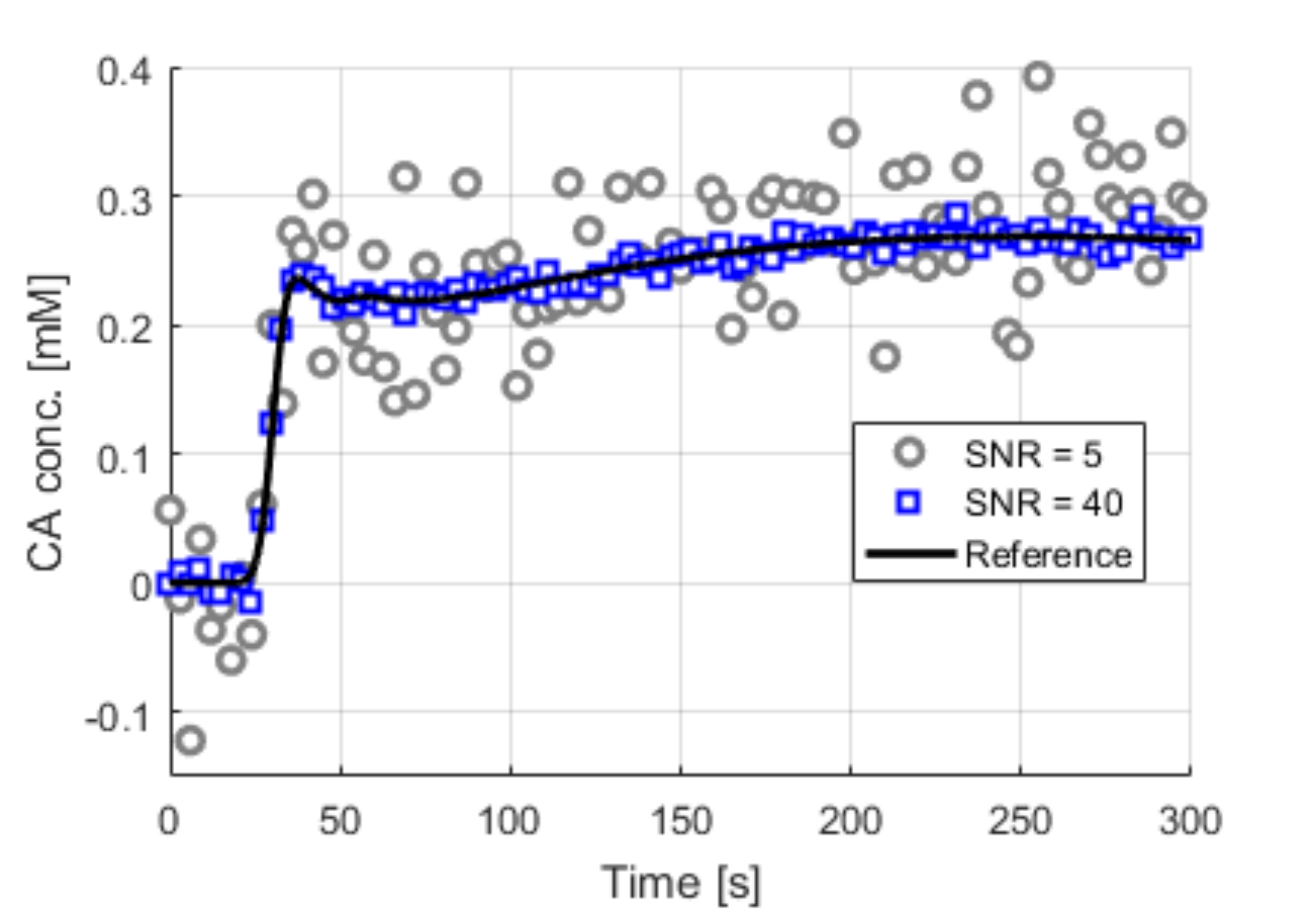
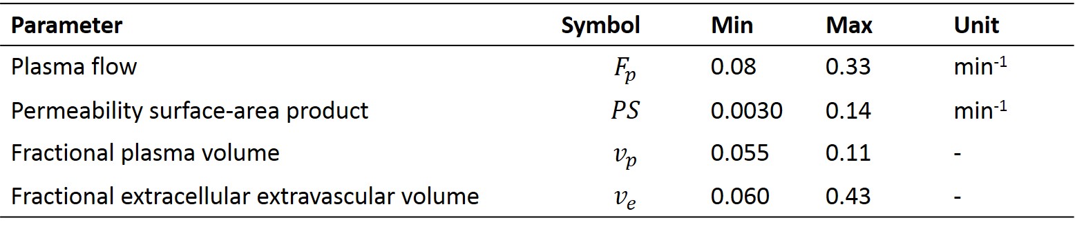
A simulation was constructed, to evaluate the performance of the WTLS estimator for the 2CXM. High temporal resolution tissue curves and arterial input curves of duration 5 min were generated for PK parameters corresponding to head-neck tumors9. The parameter values were picked at random in the range shown in Table 1, with a Gaussian probability distribution centered at the center of the range and with a standard deviation corresponding to 25% of the range for each parameter. Simulated measured curves were obtained at several different noise levels by sampling to 3 s resolution and adding Gaussian noise. Figure 1 shows two example curves corresponding to the lowest and highest simulated SNR. PK parameters were subsequently estimated using the NLLS method, the LLS method3 and the proposed WTLS method.
For each noise level, method, and parameter in the 2CXM, the relative error in each parameter was evaluated for 10000 simulations as $$e_i = \frac{\hat{p}_i-p_i}{p_i}$$ where $$$\hat{p}_i$$$ and $$$p_i$$$ correspond to the estimated and true parameters in the 2CXM. Relative accuracy and precision were evaluated from the errors $$$e_i$$$ as the median value and the distance between the 5th and 95th percentiles, respectively.
Results
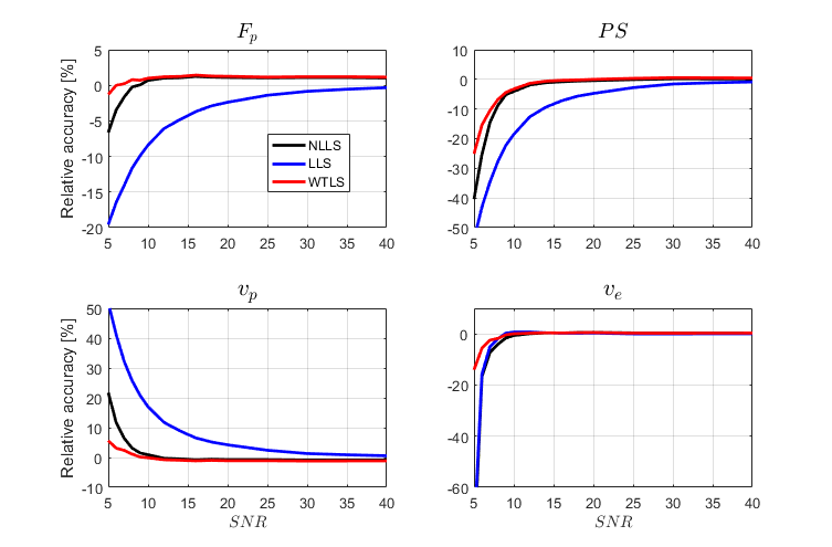
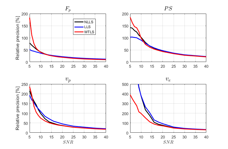
The accuracy as a function of SNR (defined as maximum tissue CA concentration over noise standard deviation) for the four model parameters in the 2CXM, is shown in Figure 2. Similarly, Figure 3 shows the precision. The average time to fit a single curve was 2.8 ms for the NLLS method, 0.10 ms for the LLS method, and 1.2 ms for the proposed WTLS method.Discussion and Conclusions
The main finding in this work is that the bias introduced when using LLS to estimate parameters from the 2CXM can be reduced by taking the statistics of the noise into account with a WTLS estimator. Except at low SNR (< 10) the precision is also improved, but only slightly. At SNR < 10, the results for the precision were less coherent, with improved precision for some parameters and worse precision for other.
An important motivation for the development of LLS methods is computational speed. Unfortunately, a large part of this speed advantage is lost with the WTLS estimator due to the need for a Cholesky decomposition of $$$WW^T$$$ (or some other methods to invert this matrix). Thus, to obtain both speed and accuracy, future research should focus on speeding up the WTLS estimator by for instance developing approximations of the $$$(WW^T)^{-1}$$$ term.
Acknowledgements
No acknowledgement found.References
1. Sourbron SP, Buckley DL. Tracer kinetic modelling in MRI: estimating perfusion and capillary permeability. Phys. Med. Biol. 2012;57:R1–33.
2. Murase K. Efficient method for calculating kinetic parameters using T1-weighted dynamic contrast-enhanced magnetic resonance imaging. Magn. Reson. Med. 2004;51:858–62.
3. Flouri D, Lesnic D, Sourbron SP. Fitting the two-compartment model in DCE-MRI by linear inversion. Magn. Reson. Med. 2016;76:998–1006.
4. Kallehauge JF, Sourbron S, Irving B, Tanderup K, Schnabel JA, Chappell MA. Comparison of Linear and Nonlinear Implementation of the Compartmental Tissue Uptake Model for Dynamic Contrast-Enhanced MRI. Magn. Reson. Med. 2016. doi: 10.1002/mrmt.26324.
5. Wen L, Eberl S, Fulham MJ, Feng D, Bai J. Constructing reliable parametric images using enhanced GLLS for dynamic SPECT. IEEE Trans. Biomed. Eng. 2009;56:1117–1126.
6. Varga J, Szabo Z. Modified regression model for the Logan plot. J. Cereb. Blood Flow Metab. 2002;22:240–4.
7. Dai X, Chen Z, Tian J. Performance evaluation of kinetic parameter estimation methods in dynamic FDG-PET studies. Nucl. Med. Commun. 2011;32:4–16.
8. Markovsky I, Van Huffel S. Overview of total least-squares methods. Signal Processing 2007;87:2283–2302.
9. Donaldson SB, Betts G, Bonington SC, Homer JJ, Slevin NJ,
Kershaw LE, Valentine H, West CML, Buckley DL. Perfusion estimated with rapid
dynamic contrast-enhanced magnetic resonance imaging correlates inversely with
vascular endothelial growth factor expression and pimonidazole staining in
head-and-neck cancer: A pilot study. Int. J. Radiat. Oncol. Biol. Phys.
2011;81:1176–1183.
Figures