Synopsis

One of the most demanding challenges with ultra-high field MRI is the SAR_10g assessment during a multi-channel transmit MRI examination. A worst-case estimate is often used. In this work a fast method is presented to assess the upper bound of the maximum SAR_10g for body coil arrays with knowledge on only the power distribution among the channels. The performance is assessed for prostate imaging at 7T using our database with 23 realistic subject-specific models. The mean overestimation factor is 1.58 and the mean reduction in overestimation is 0.75 compared to a recently presented alternative estimation method.

Purpose

Methods

With multi-channel transmit systems the worst-case $$$SAR_{10g}^{WC}$$$ equals the maximum eigenvalue multiplied with the square of the norm of the drive vector $$$I$$$.

$$SAR_{10g}^{WC}= \max_j({\lambda_{max}}^j)||I||_2^2$$

Where, $$${\lambda_{max}}^j$$$ is the maximum eigevalue of the $$${Q_{10g}}^j$$$ matrix of the voxel $$$j$$$, $$$I=[i_1,i_2,...,i_{Ne}]^T$$$ is the drive vector which contains the current $$$i_n$$$ transmitted by each channel and $$$Ne$$$ is the number of channels.

This worst-case upper bound assumes a drive vector equal or proportional to the eigenvector associated to the maximum eigenvalue, resulting in an overly conservative overestimation in many cases. When the amplitudes of the channels are known, an optimization method to approximate the maximum SAR_10g has recently been published by Orzada et al.³. However, this method requires arbitrary reference phases, many iterations and random starting points making the process long and non-deterministic.

We present an alternative upper bound. For each voxel $$$j$$$ the Q-matrix is setup by an E-field multiplication:

$${q_{n,m}}^j=\frac{\sigma^j}{2\rho^j}\left\{({E_{x,n}}^j)^*{E_{x,m}}^j+({E_{y,n}}^j)^*{E_{y,m}}^j+({E_{z,n}}^j)^*{E_{z,m}}^j\right\}$$

where $$${E_{x,n}}^j$$$, $$${E_{y,n}}^j$$$ and $$${E_{z,n}}^j$$$ are the $$$x$$$,$$$y$$$, and $$$z$$$-components of the E-field generated by the $$$n$$$-th array element at voxel $$$j$$$. Assuming that the $$$z$$$-component is dominant, which is true for many arrays including the on-body dipole array in this study:

$${q_{n,m}}^j=\frac{\sigma^j}{2\rho^j}({E_{z,n}}^j)^*{E_{z,m}}^j=\frac{\sigma^j}{2\rho^j}({E_{n}}^j)^*{E_{m}}^j$$

Then the $$$SAR^j$$$ is given by:

$$SAR^j=\sum_{n=1}^{Ne}\sum_{m=1}^{Ne}i_n^*{q_{n,m}}^ji_m=\frac{\sigma^j}{2\rho^j}\sum_{n=1}^{Ne}\sum_{m=1}^{Ne}i_n^*({E_{n}}^j)^*{E_{m}}^ji_m$$

This expression is maximized with respect to the input phases for $$$i_n=|i_n|e^{-\phi({E_n}^j)}$$$ and $$$i_m=|i_m|e^{-\phi({E_m}^j)}$$$:

$${SAR_{max}}^j=\frac{\sigma^j}{2\rho^j}\sum_{n=1}^{Ne}\sum_{m=1}^{Ne}|i_n|e^{\phi({E_n}^j)}|{E_{n}}^j|e^{-\phi({E_n}^j)}|{E_{m}}^j|e^{\phi({E_m}^j)}|i_m|e^{-\phi({E_m}^j)}=\frac{\sigma^j}{2\rho^j}\sum_{n=1}^{Ne}\sum_{m=1}^{Ne}|i_n||{E_{n}}^j||{E_{m}}^j||i_m|=\frac{\sigma^j}{2\rho^j}\sum_{n=1}^{Ne}\sum_{m=1}^{Ne}|i_n||({E_{n}}^j)^*{E_{m}}^j||i_m|$$

The last term equals:

$${SAR_{max}}^j=\sum_{n=1}^{Ne}\sum_{m=1}^{Ne}|i_n||{q_{n,m}}^j||i_m|$$

We now assume that averaging the SAR over 10g will still result in maximum SAR_10g for these drive vector phases. The maximum SAR_10g that can be reached for all voxels is:

$$SAR_{10g}^{UB}=\max_j\left(\sum_{n=1}^{Ne}\sum_{m=1}^{Ne}|i_n||{q_{n,m}}^j||i_m|\right)$$

This upper bound can be evaluated for the Q-matrix of each individual voxel or using the Q-matrices that correspond to the VOPs² to reduce the calculation time.

To evaluate the performances, the proposed upper bound ($$$SAR_{10g}^{UB}$$$) is compared with the worst-case upper bound ($$$SAR_{10g}^{WC}$$$) and with the optimized upper bound³ ($$$SAR_{10g}^{OPT}$$$) using our database with 23 realistic subject-specific pelvis models. The VOP method² is used to calculate the maximum SAR ($$$SAR_{10g}^{VOPs}$$$) for 10000 random drive vectors (with uniform and non-uniform amplitudes). We assume that this samples the whole feasible SAR space allowing to determine the overestimation factor of each upper bound method.

Results and Discussion

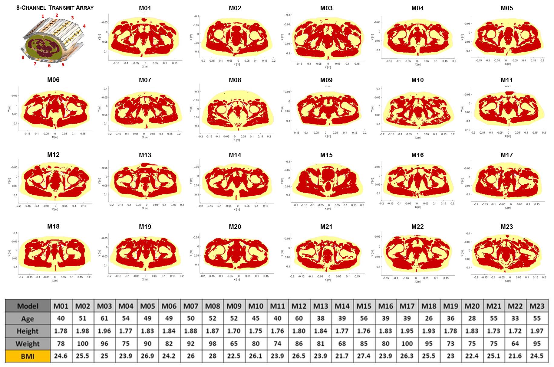
In Fig.1 the 8-channel fractionated dipole array for prostate imaging is shown and the 23 body models of the pelvic region⁴.

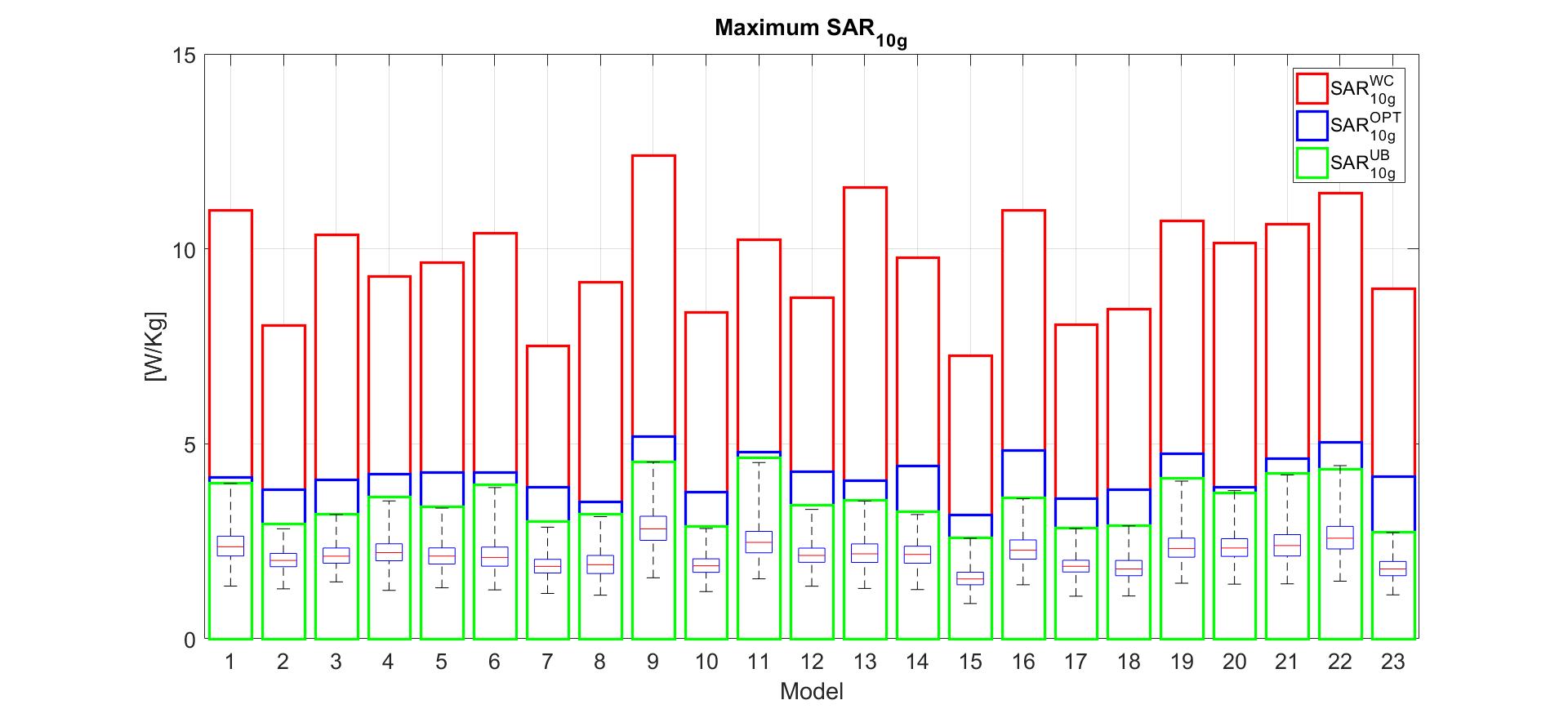
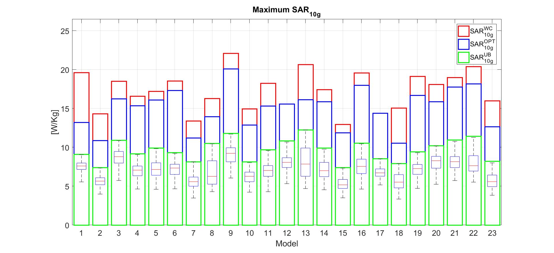
Fig.2 shows the $$$SAR_{10g}^{UB}$$$, $$$SAR_{10g}^{WC}$$$, $$$SAR_{10g}^{OPT}$$$ and the statistics of the estimated $$$SAR_{10g}^{VOPs}$$$ for each model with drive vectors with uniform amplitudes and random phases. Fig.3 shows the upper bounds and the $$$SAR_{10g}^{VOPs}$$$ statistics for drive vectors with non-uniform amplitudes and random phases. The observed maximum $$$SAR_{10g}^{VOPs}$$$ is always very close to $$$SAR_{10g}^{UB}$$$ and in some cases is slightly higher than it, thus showing an overestimation lower than the allowed VOP overestimation (5% maximum overestimation).

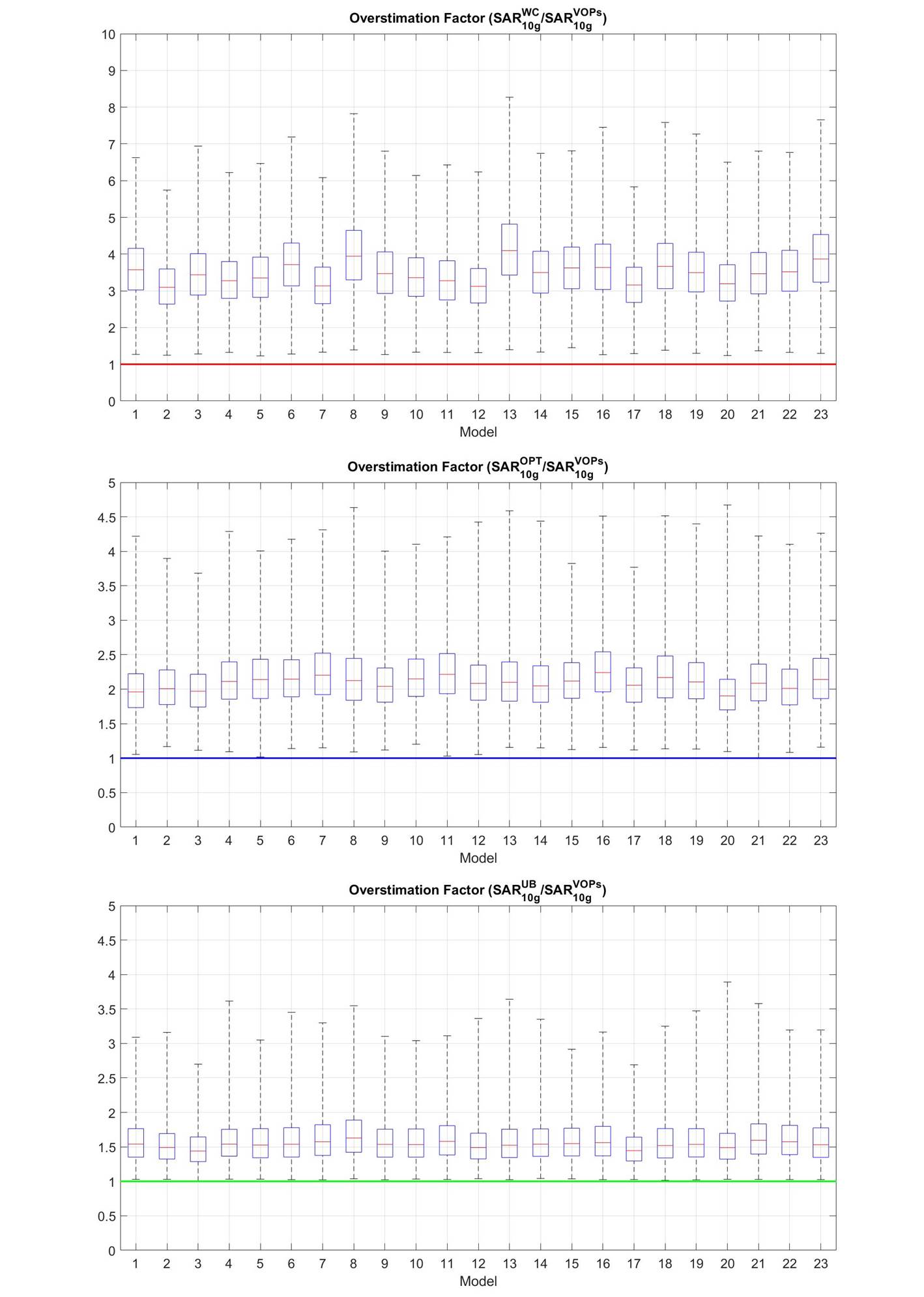
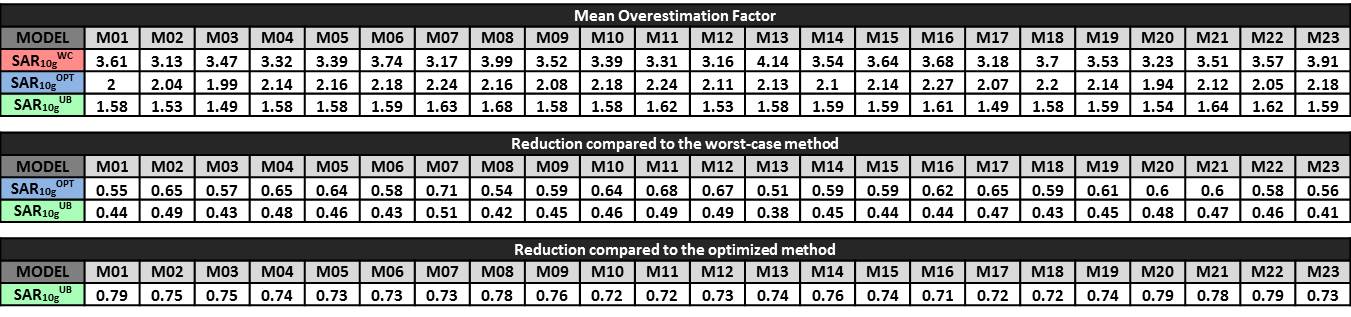
In Fig.4 the statistics of the overestimation factors with drive vectors with random amplitudes and phases are reported. As highlighted in Tab.1, the mean overestimation factors are between 3.13-4.14 for $$$SAR_{10g}^{WC}$$$, between 1.94-2.27 for $$$SAR_{10g}^{OPT}$$$ and between 1.49-1.68 for $$$SAR_{10g}^{UB}$$$. Using $$$SAR_{10g}^{UB}$$$ the reductions in the overestimation compared to $$$SAR_{10g}^{WC}$$$ are between 0.38-0.51. Compared to $$$SAR_{10g}^{OPT}$$$ are between 0.71-0.79.

The indicated overestimation factors are representative for on-body dipole arrays or other setups where only one component of the electric field distribution is dominant at the locations where the maximum SAR may occur. This assumption is valid in our case.

Conclusions

Acknowledgements

References

[1] I. Graesslin, H. Homann, S. Biederer, P. Börnert, K. Nehrke, P. Vernickel, G. Mens, P. Harvey, U. Katscher, A specific absorption rate prediction concept for parallel transmission MR. Magn Reson Med. 2012 Nov;68(5):1664-74.

[2] G. Eichfelder and M. Gebhardt, Local Specific Absorption Rate Control for Parallel Transmission by Virtual Observation Points, Magn. Reson. Med. 2011, vol. 66, no. 5, pp. 1468-1476.

[3] S. Orzada, M.E. Ladd, A.K.Bitz, A method to approximate maximum local SAR in multichannel transmit MR systems without transmit phase information, Magn Reson Med. 2016 Sep 8. doi: 10.1002/mrm.26398.

[4] E.F.Meliado, A.J.E Raaijmakers, M.C. Restivo, M. Maspero, P.R. Luijten, C.A.T. van den Berg, Database Construction for Local SAR Prediction: Preliminary Assessment of the Intra and Inter Subject SAR Variability in Pelvic Region, Proceedings of the ISMRM 24th Annual Meeting, Singapore, 7-13 May 2016.

[5] A.J.E. Raaijmakers, M. Italiaander, I.J. Voogt, P.R. Luijten, J.M. Hoogduin, D.W.J. Klomp, C.A.T. van den Berg. The fractionated dipole antenna: A new antenna for body imaging at 7 Tesla. Magn Reson Med. 2015 May 2 : 10.1002/mrm.25596. Published online 2015 May 2. doi: 10.1002/mrm.25596.