Introduction

Portable MRI scanner is an attractive option for medical imaging for their merits of compact size, light weight, and low price. Permanent magnet is a popular option to provide the main magnetic field for portable MRI scanners due to its low cost, no electric power consumption, and low fringe field. However, it is challenging to build a permanent magnet array generating a strong yet homogeneous magnetic field over a large volume for parts of human body, such as the human head. Here, we propose an effective and fast optimization method for the design of permanent magnet arrays. Both magnets and iron blocks are considered as building blocks.

Methods

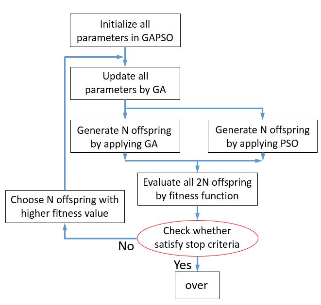
The proposed design procedure of a permanent magnet array includes two parts: the calculation of magnetic fields and the optimization. Magnetic Field Calculation: Boundary integral method (BIM) is implemented to calculate the magnetic fields^1-3. A scalar potential $$$φ$$$ is introduced, set $$$\small\overline{H}=-\nabla\varphi$$$ (1). Combine (1) with Maxell’s equations, $$$\small\overline{B}$$$ can be expressed as: $$$\small\overline{B}(\overline{r})=\frac{\mu_0}{4\pi}\int_{v'}\frac{(\overline{r'}-\overline{r})\nabla'\bullet\overline{M}(\overline{r'})}{|\overline{r}-\overline{r'}|^3 }dv'-\frac{\mu_0}{4\pi} \oint_{s'}\frac{(\overline{r}'-\overline{r})\bullet(\overline{M}(\overline{r'})\bullet\overline{n})}{|\overline{r}-\overline{r'}|^3}ds'$$$ (2). In equation (2), $$$\small{ν'}$$$ is a closed domain with boundary $$$\small{s'}$$$, and $$$\small\overline{M}(\overline{r'})$$$ is the magnetization. $$$\small\overline{r}$$$ is the observation point, and $$$\small\overline{r'}$$$ is the source point. $$$\small\overline{n}$$$ is the normal vector perpendicular to the surface $$$\small{s'}$$$ pointing outside the domain $$$\small{v'}$$$. $$$\small\overline{M}(\overline{r'})$$$ is assumed to be uniform in domain $$$\small{v'}$$$, thus the first integral in (2) vanishes, and $$$\small\overline{B}(\overline{r})$$$ is written as: $$$\small\overline{B}(\overline{r})=Q(\overline{r})\bullet\overline{M}(\overline{r'})$$$ (3), and $$$\small{Q}(\overline{r})\frac{\mu_0}{4\pi}\oint_{s'}\frac{(\overline{r}-\overline{r'})\otimes\overline{n}}{|\overline{r}-\overline{r'}|^3} ds'$$$ (4). For magnets, $$$\small\overline{M}(\overline{r})$$$ is known and $$$\overline{B}(\overline{r})$$$ can be easily calculated. However, for irons, $$$\small\overline{M}(\overline{r})$$$ is unknown and is determined by both the interaction between magnets and irons and that among irons themselves. $$$\small\overline{B}$$$ and $$$\overline{M}$$$ at the center of the $$$\small{i}_{th}$$$ iron is labeled as $$$\small\overline{B}_i$$$ and $$$\small\overline{M}_i$$$, so $$$\small\overline{B}_i$$$ can be expressed as: $$$\small\overline{B}_i=\sum_{k=1}^N{Q}_{ik}\bullet\overline{M}_k+\overline{B}_{exi},i=1,2,3\cdots{N}$$$ (5), where $$$\small{Q}_{ik}$$$ is the interaction matrix caused by the $$$\small{k}_{th}$$$ iron at the center of the $$$\small{i}_{th}$$$ iron. $$$\small\overline{B}_{exi}$$$ is the field caused by all magnets at the center of the $$$\small{i}_{th}$$$ iron and can be calculated by $$$\small\overline{B}_{exi}=\sum_{l=1}^N{Q}_{il}\bullet\overline{M}_l,{i}=1,2,3\cdots{N}$$$ (6), where $$$\small\overline{M}_l$$$ is the remanent magnetization of the $$$\small{l}_{th}$$$ magnet. If we set $$$\small\overline{M}_i=f(\overline{B}_i),{i = 1, 2, 3\cdots{N}}$$$ (7), $$$\small\overline{B}_i$$$ can be solved by an iterative procedure. For the $$$\small{p}_{th}$$$ step in the iterative procedure, equation (5) and (6) can be written as $$$\small\overline{B}_i^p=[E-{Q}_{ii}\bullet f(\overline{B}_i^{p-1})]^{-1}\bullet(\sum_{k=1}^{i-1}{Q}_{ik}\bullet\overline{M}_i^P+\sum_{k'=i+1}^{N}{Q}_{ik'}\bullet\overline{M}_{k'}^{p-1}+\overline{B}_{exi})$$$ (8). The iterative procedure is stopped when $$$\small\overline{M}_i^p$$$ is stable. So after the iterative procedure, $$$\small\overline{M}$$$ of the irons is solved, and $$$\small\overline{B}$$$ at the observation points can be computed by (3) and (4). BIM does not require to discretize free space between magnets and irons thus it requires less segmentations and less unknowns. Consequently, it has higher computational efficiency than a conventional approach, e.g. finite element method (FEM). Optimization Algorithm: The optimization procedure is implemented by applying genetic algorithm particle swarm optimization (GAPSO). GAPSO combines the PSO’s swam intelligence and GA’s natural selection. As a result, these advantages make GAPSO have high-diversity potential solutions and quick solution-seeking speed.⁴ The flowchart of GAPSO is shown in Fig. 1. The optimization of the homogeneity and the strength of the magnetic field is achieved by both optimizing the configuration of the main magnet array and by introducing small iron parts at locations surrounding the magnet array.

Results

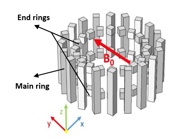
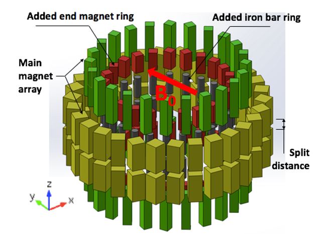
The optimization is based on the design shown in Fig. 2.⁵ As shown in Fig. 2, the magnet bars are located with a distance apart. The distance between successive bars is optimized to eliminate the end effects caused by the finite length of bars. The volume of interest (VOI) is a cylindrical one with a diameter of 200 mm and a length of 50 mm. The magnets are N52 grade NdFeb. The optimized configuration of the array is shown in Fig. 3.

Discussions

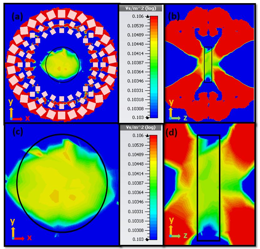
The optimization results are verified in CST⁶ and are shown in Fig. 4. The Lamor frequency bandwidth in VOI is optimized from over 500 KHz (over 120000 ppm) to 63.47 KHz (about 14200 ppm), a reduction of 88.2%. In the meanwhile, the field strength is increased by 59.0% from 66 mT to 105 mT. The variations of the magnetization of the magnets should be taken in account in the future.

Conclusions

We present an effective and fast optimization method for magnet array design by applying BIM for the calculation of magnetic field with high computational efficiency and GAPSO for optimization with highly diversified options and high convergence rate. The effectiveness of optimization is validated by simulated results. The optimized magnet array will be built for low-field MR imaging where spatial encoding strategy is applied for imaging.⁷

Acknowledgements

This research was supported by SUTD President's Graduate Fellowship. I would like to take this opportunity to express my sincere gratitude for their support.