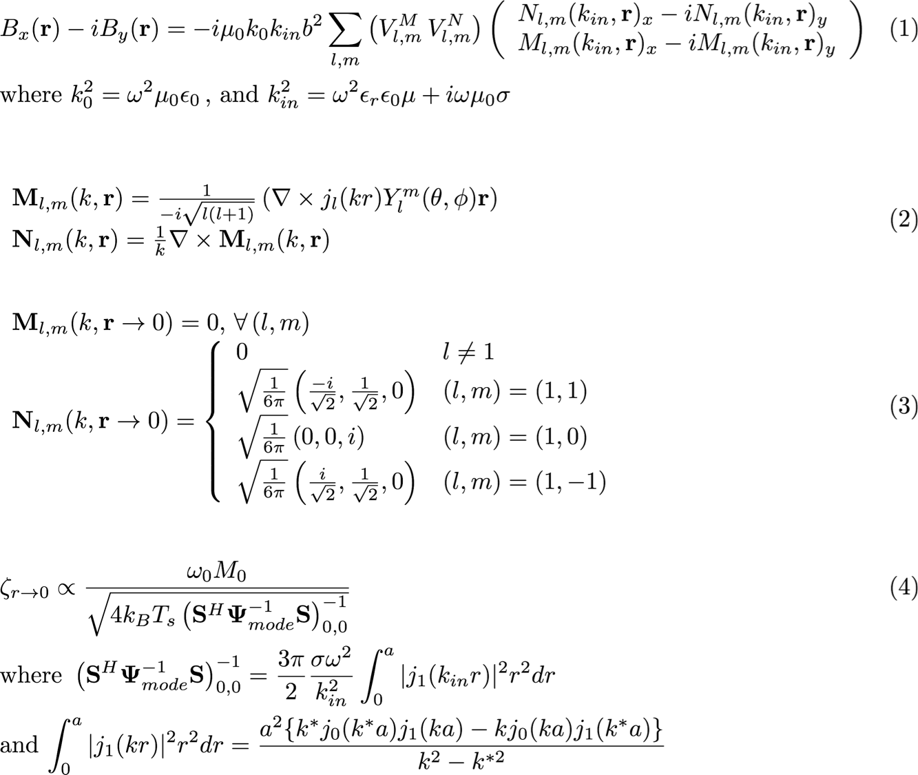
4293
An analytic expression for the ultimate intrinsic SNR in a uniform sphere1Center for Biomedical Imaging, New York University, New York, NY, United States
Synopsis
Ultimate intrinsic SNR (UISNR) is the theoretically highest SNR for given geometry and electrical properties, independent of the coil design. Here, we introduce an analytic exact expression to calculate the UISNR at the sphere center, enabling to directly analyze the dependence on main magnetic field, sample geometry and electric properties. The analytic expression can approximate the UISNR near the center with < 5% error. This work can enable people without access to the full simulation code to calculate UISNR and use it, for example, as an absolute reference to assess the performance of head coils with spherical phantoms.
Purpose
Ultimate intrinsic signal-to-noise ratio (UISNR) is the theoretically largest SNR for given sample geometry and electrical properties, independent of coil design [1-4]. UISNR can be calculated via a current mode expansion and dyadic Green's functions (DGF) [5,6]. Only few modes contribute to the UISNR in the central region of a uniform sphere, compared to thousands of modes at other voxel positions [4,7]. Based on this previous observation, the aim of this work was to derive an analytic expression for the UISNR $$$\zeta_{r\to0}$$$ at the center of a sphere.Theory and Methods
All equations are defined in Fig.1. The receive sensitivity $$$B_x(r)-iB_y(r)$$$ (Eq.(1)) inside a dielectric sphere of radius $$$a<b$$$, where $$$b$$$ is the radius of the surface where the current modes are defined, is determined by the vector wave functions $$$M_{l,m}$$$ and $$$N_{l,m}$$$ (Eq.(2)).
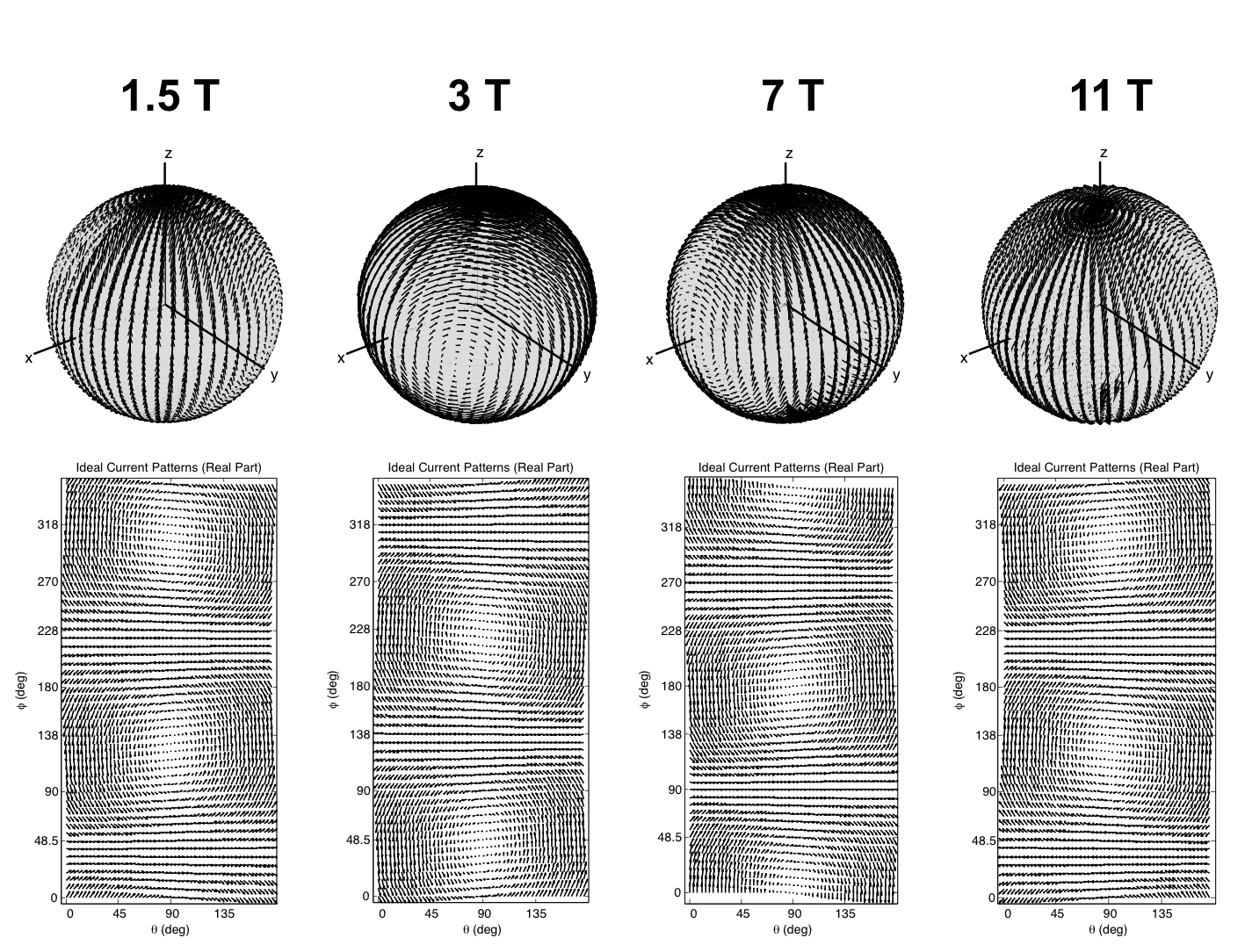
At the sphere center ($$$r\to0$$$), we found that $$$M_{l,m}(r\to0)=0$$$ $$$\forall (l,m)$$$ and $$$N_{l,m}(r\to0)=0$$$ $$$\forall (l,m)$$$, except $$$N_{1,1}$$$, $$$N_{1,0}$$$, and $$$N_{1,-1}$$$ (Eq.(3)). Substituting Eq.(3) into Eq.(1), we see that only $$$N_{1,1}$$$ contributes to the receive sensitivity at the center, meaning that the corresponding UISNR ($$$\zeta_{r\to0}$$$) is completely determined by one divergence-free current mode. This explains why the corresponding shape of the ideal current patterns [5] does not change with field strength (Fig.2), and indicates that loops are the optimal coil elements to maximize central SNR.
The analytic expression for $$$\zeta_{r\to0}$$$ is given in Eq.(4), which explicitly shows the dependence of $$$\zeta_{r\to0}$$$ on radius and wave number (electrical properties) of the dielectric sphere.
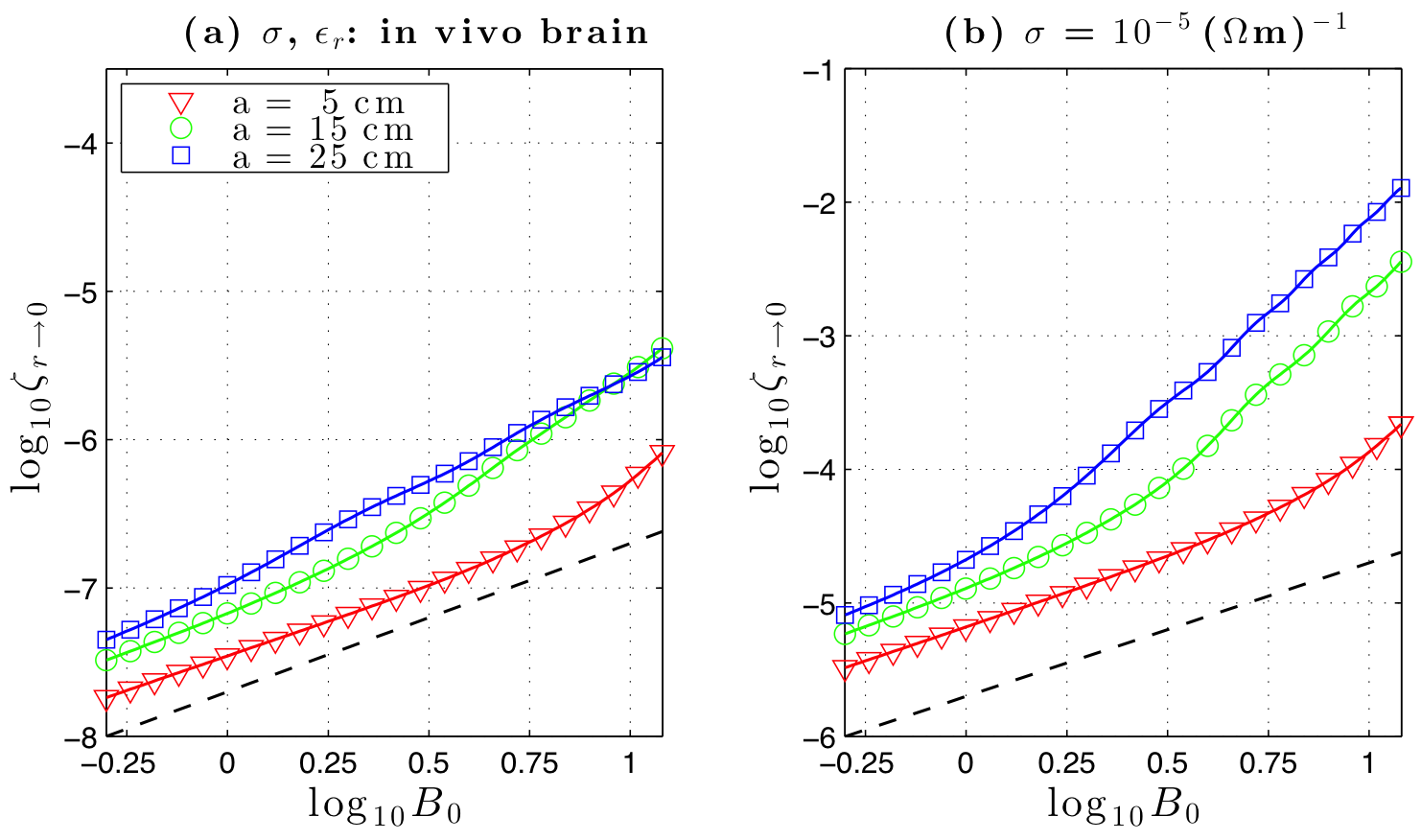
To validate the analytic solution, we investigated the dependence of $$$\zeta_{r\to0}$$$ on main magnetic field strength $$$B_0$$$ and compared the results with corresponding DGF simulation results, with expansion order $$$l_{max}=55$$$. Average brain tissue was used for the dielectric properties of the sphere, $$$\epsilon_r$$$ and $$$\sigma$$$ [4]. We also tested the case with conductivity $$$\sigma$$$ equals to $$$10^{-5}(\Omega^{-1}m^{-1})$$$ to approximate the lossless condition as in Ref. [4].
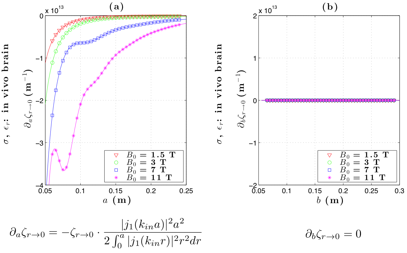
We used the analytic expression to study the dependence of $$$\zeta_{r\to0}$$$ on the sphere radius ($$$a$$$) and the radius of the surface where the current distribution is defined ($$$b$$$).
Finally, we investigated how the UISNR ($$$\zeta_r$$$) varies with the distance $$$r$$$ from the center, either along the x-y plane or z-axis ($$$B_0$$$ direction), and determined the range for which the UISNR can be approximated by the value at the center ($$$\zeta_{r\to0}$$$).
Results and Discussion
Fig.3 shows the double-logarithmic plots of $$$\zeta_{r\to0} vs. B_0$$$ for $$$B_0$$$=0.5-12 T, replicating the plots in fig.6 of Ref. [4]. The $$$\zeta_{r\to0}$$$ based on the analytic solution (solid lines) was consistent with the results in Ref. [4], which used a multipole expansion to calculate UISNR, and also with values calculated with full DGF simulations (data points). Fig.3 shows that $$$\zeta_{r\to0}$$$ is approximately linear with respect to $$$B_0$$$ at low $$$B_0$$$ and increase nonlinearly ~$$${B_0}^n$$$ with an exponent $$$n>1$$$ at high $$$B_0$$$, compatible to published results [4].
The sensitivity of the central UISNR with respect to changes in sphere radius ($$$\partial_a\zeta_{r\to0}$$$) and current radius ($$$\partial_b\zeta_{r\to0}$$$) is shown in Fig.4. The analytic results (solid lines) agree with those from DGF simulations (data points). The UISNR at the center grows monotonically with sphere radius until reaching a plateau (Fig.4a), except at 11 T, where its value oscillates for small sphere radii, likely due to wavelength effects. Intuitively, since there are no conductive losses in air, $$$\zeta_{r\to0}$$$ should not depend on the radius at which the current distribution is defined ($$$b$$$). This is, in fact, confirmed by the analytic expression (Eq.(4)) and by Fig. 4b, where $$$\partial_b\zeta_{r\to0}=0$$$.
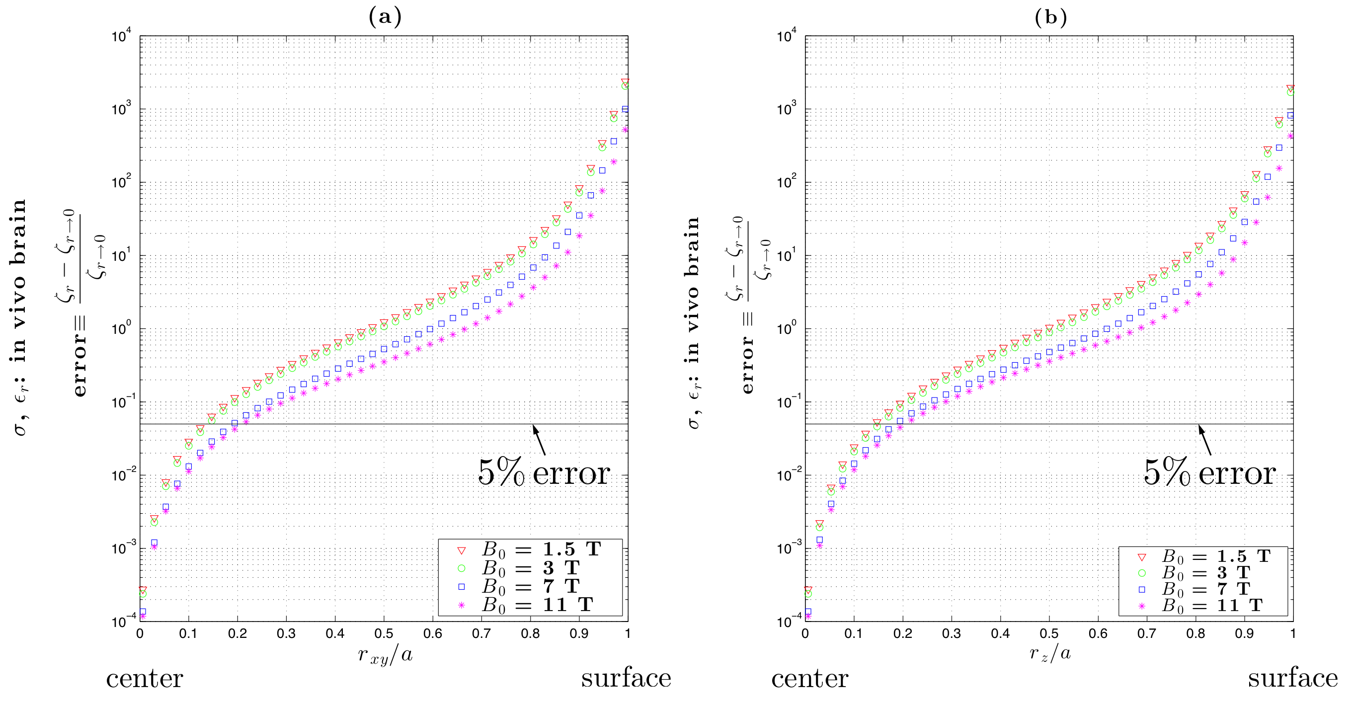
Fig.5 shows that using the UISNR at the center to approximate the UISNR for a voxel at an intermediate position (0<$$$r/a$$$<1) on the x-y plane (Fig. 5a), or z-axis (Fig. 5b) yields an error <5% if $$$r/a$$$<10-20%.
While an approximate solution, with very limited validity, had been proposed for the UISNR [8], our analytic solution of $$$\zeta_{r\to0}$$$ is exact and consistent to full simulations. Calculation speed is 800 times faster than for full simulations.
Conclusion
We introduced an analytic expression to calculate the UISNR at the center of a dielectric sphere, which is rapid, accurate, and enables to directly analyze the dependence on $$$B_0$$$, sample geometry and electric properties. The analytic expression can approximate the UISNR near the center with an acceptable error: for a typical spherical phantom with radius = 8.5cm, the UISNR would be valid within a central volume of ~(2cm)$$$^3$$$. This work can enable people without access to the full simulation code to calculate UISNR and use it, for example, as an absolute reference to assess the performance of head coils with spherical phantoms [9].Acknowledgements
This work was performed under the rubric of the Center for Advanced Imaging Innovation and Research (CAI2R, www.cai2r.net), a NIBIB Biomedical Technology Resource Center (NIH P41 EB017183).References
[1] Ocali, O. & Atalar, E. (1998) MRM 39,462–473.
[2] Schnell, W., et al. (2000) IEEE Trans. Antennas. Propag. 48(3),418-428
[3] Ohliger, M.A., et al. (2003) MRM 50,1018-1030
[4] Wiesinger, F., et al. (2004) MRM, 52:376-390.
[5] Lattanzi, R. & Sodickson, D.K. (2012) MRM, 68:286-304.
[6] Vaidya, M.V., et al. (2014) Concepts Magn. Reson. B Magn. Reson. Eng., 44(3):53-65.
[7] Lattanzi, R., et al. (2012) Proc. ISMRM, 20, 2817.
[8] Kopanoglu, E., et al. (2011) MRM, 66:846-858.
[9] Lattanzi, R., et al. (2010) NMR Biomed. 23(2),142-151.
Figures