Synopsis

A complete MRI RF simulation has at least two parts involved: S-parameter optimization including frequency tuning, impedance matching and channel decoupling, and RF field generation. Previous EM-Circuit co-simulation work used every port data for field synthesis. In this abstract, the speeding factor, or the CPU/GPU time reduction factor, of the co-simulation method against the traditional broadband calculation, is present. We also compared the accuracy of field synthetization from every port data, vs. from every channel data, and propose a highly automatic optimal simulation flow that offers best field accuracy, minimum computer disk space and memory requirement, and fast data processing.

Purpose

Methods

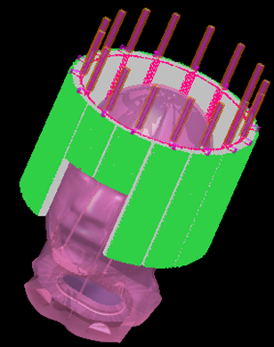
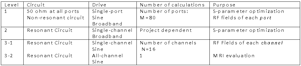
A 7T 16-ch stripline head array (Fig. 1) ^5-6 was simulated with FDTD method (xFDTD, Remcom, USA), on a linux system using GPUs (4 T10 in an S1070, NVIDIA, USA). All simulation converged to -50dB. Circuit optimization aimed at finding optimum values of lumped elements was done with SOMA³.

Description of the EM simulations performed in this study is provided in Table 1. For S-parameter optimization we considered two methods: 1) broadband simulation of each transmit channel to emulate the bench procedure with a Network/Spectrum Analyzer (defined as “Broadband 2”) and 2) co-simulation using a sinusoidal drive for each port (defined as “Sine 1”).

After obtaining the optimum values of lumped elements, we compared three approaches to generate the final RF fields for a given transmit configuration: 1) direct synthesis using port-specific field maps obtained from simulation Sine 1 (defined as “Synthesis 1”), 2) synthesis using multi-channel field maps obtained from simulation Sine 3-1 in which channel-specific field maps were calculated by full EM simulation (defined as “Synthesis 2”) and 3) full EM simulation of the final field (ie, simulation Sine 3-2).

Two transmit configurations were considered: 1) quadratic phases and 2) modified phases that presented larger phase changes between neighboring transmit channels. The phases in degrees utilized in the modified phase configuration were: 79.61,-57.78, 36.03, -12.17, -12.17, 36.03, -57.68, 79.61, 100.39, 122.32, 56.00, 167.83, 90.00, -143.97, -60.00, -100.39. For both configurations, the three approaches to field generation were tested and compared.

Results

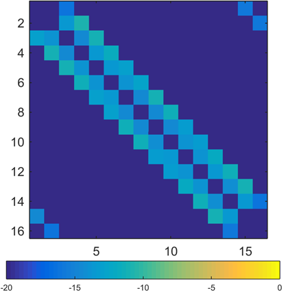
Both S-parameter optimizations gave rise to almost identical results (Fig.2). However, a single Sine 1 simulation converging to -50dB was on average 30-fold faster than a single Broadband 2 simulation, and required little human invention.

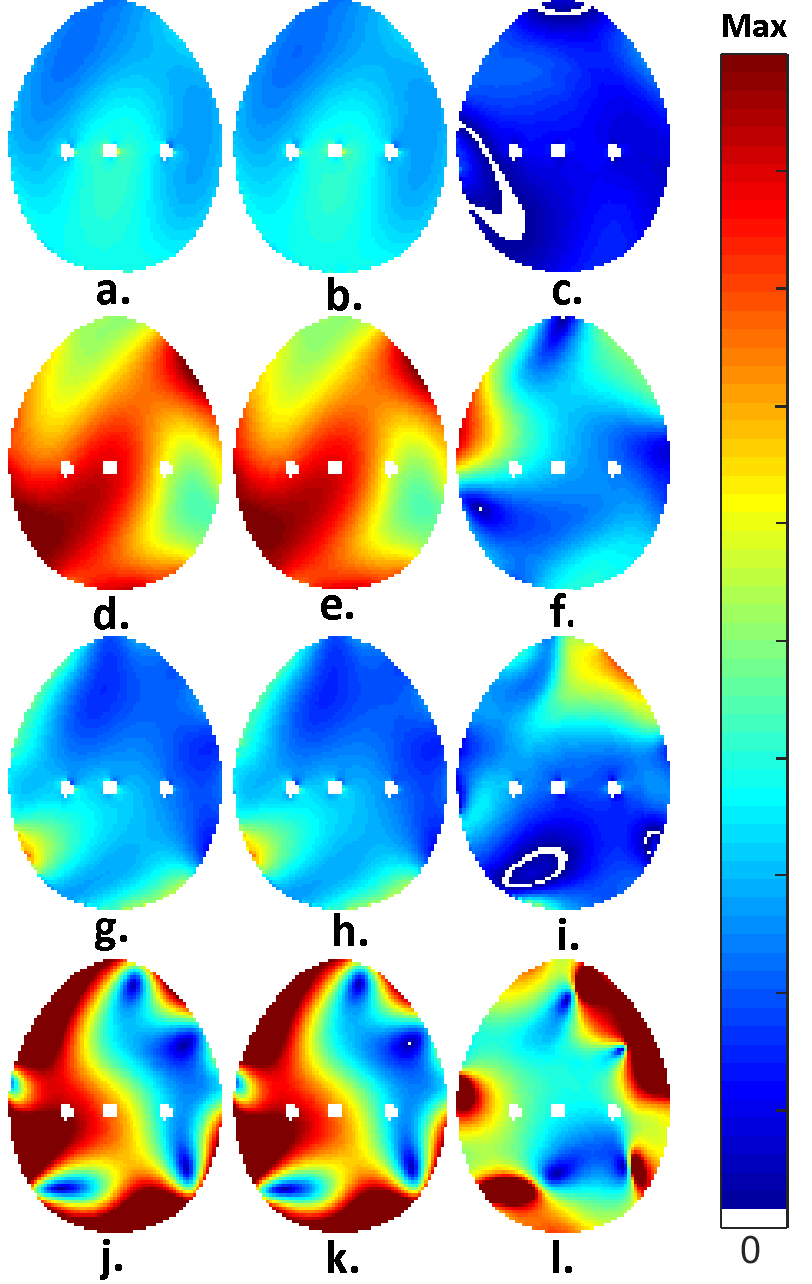
All three methods considered for field synthetization produced similar field patterns (Fig. 3). Taking the full EM simulation as a groundtruth, the co-simulation method (ie, “Synthesis 1”) led to larger errors in field synthetization than the “Synthesis 2” method. Quantitatively, when comparing |E| fields, the max relative error of the co-simulation method was 2.6% in transmit configuration 1 and 7.9% in transmit configuration 2; for |B₁⁺| comparison, the error was 9.1% in configuration 1 and 10% in configuration 2. By contrast, in all cases, the errors of the “Synthesis 2” method were less than 1%.

While reducing data quantity by 80% (16 vs. 80 3D datasets), the “Synthesis 2” method had to spend time on full EM simulation of each transmit channel, resulting in doubled GPU time as compared to the co-simulation method.

Conclusions

1). In agreement with previous work, co-simulation can be used to substantially reduce the computation time for S-parameter optimization, as compared with the traditional Broadband 2 simulations. However following conventional co-simulation procedure and synthesizing the final field by combining port-specific field maps can result in large errors as compared to a full EM of a given transmit configuration. For better accuracy, one could consider to synthesize the final field by first simulating channel-specific field maps of individual transmit channels.

2). For best accuracy, minimum disk space and memory requirement, and fast data processing, Sine 3-1 channel data , instead of Sine 1 port data, should be used for RF shimming or PTX processing. It is especially important for facilities with tens of high density RF arrays, and/or with lots of RF Shimming/ PTX needs.

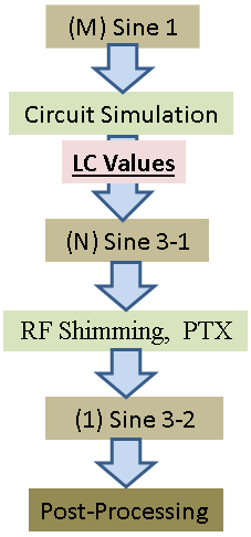
3). For high density RF arrays, we recommend the simulation flow in Fig.4. The whole procedure has (M+N+1) Sine calculations, and is highly automatic with the aid of of Matlab, including circuit simulation, RF shimming and PTX, RF fields synthesis and SAR estimation, and the production of all EM project files.

Discussions

Care should be taken when using SOMA to obtain a global optimal solution especially when many independent variables have to be optimized for channels of relative high and complex mutual couplings.

Our data suggest that field synthesis by combining port-specific field maps may result in large errors especially when transmit phases change rapidly across channels. These observations might be more meaningful for close-fitting body MRI applications with high density array, where complex transmit configurations are desired to excite in-depth organs, and |E| fields around tissue-air-metal boundary be used for SAR estimation.

Acknowledgements

References