4168
3D Parametric Histogram Analysis of Extravascular Extracellular Space for Identifying Subpopulations of Glioblastoma Related to Survival1Division of Informatics, Imaging and Data Sciences, The University of Manchester, Manchester, United Kingdom
Synopsis
Histogram Analysis of ve was used for quantification of heterogeneity in glioblastomas and to study whether heterogeneity is related to survival. 27 patients with GBM were imaged. ve histograms were processed by using a 4-mixture Gaussian distribution. Patients with short survival show an increasing proportion of the third Gaussian distribution. The mean of the 2nd Gaussian component, μ2, (p = 0.00015) and the weight of the 3rd components, w3 (p = 0.0066) were the most predictive for survival. The identification of tissue components, characterized by Gaussian fitting of ve values suggests that these represent, in some way, separate tissue subpopulations.
Purpose
In recent years there has been increasing interest in markers of
heterogeneity, particularly in glioblastoma
(GBM)
where tissue heterogeneity is a major feature. In DCE-MRI study, commonly used measurements of
parameter mean/median may not be able to fully reflect the contributions from each of the subpopulations in a
heterogeneous tumor. More dedicated histogram
analysis is therefore needed. The extravascular
extracellular space fraction (ve)
has received relatively little attention in the published literature.1 We report the
prognostic value of the ve histogram analysis, assessed in a group of patients
with GBM.Methods
27 GBM patients underwent preoperative imaging (conventional imaging and T1W DCE-MRI) on a 3T Philips Achieva MRI scanner. The patients were divided into three groups, each of nine patients, characterized by overall survival: group 1 (survival shorter than 150 days); group 2 (survival 150-365 days); group 3 (survival longer than 365 days). A hybrid approach2 was used for the kinetic analysis, which calculates vp with the First Pass model, then ve and Ktrans with the extended Tofts model. Group histograms were produced by pooling all tumor voxels for each of the three groups and normalizing by the total number of tumor voxels in the group. Group histograms were plotted the same axes to support direct comparison. Non-enhancing voxels with zero ve were excluded from the analysis. Individual histograms of ve were fitted using a mixture of Gaussian functions. The individual Gaussian probability density function (PDF) can be written as:
$$n(\chi,\mu,\sigma)=\frac{1}{\sqrt{2\pi\sigma^{2}}}\exp(-(\chi-\mu)^{2}/2\sigma^{2})$$Eq. [1]
Optimal fitting of the distribution of ve required a mixture of four Gaussians using the following expression:
$$Y=w1*n(\chi;\mu1,\sigma1)+w2*n(\chi;\mu2,\sigma2)+w3*n(\chi;\mu3,\sigma3)+w4*n(\chi;\mu4,\sigma4)$$Eq. [2]
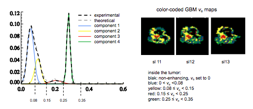
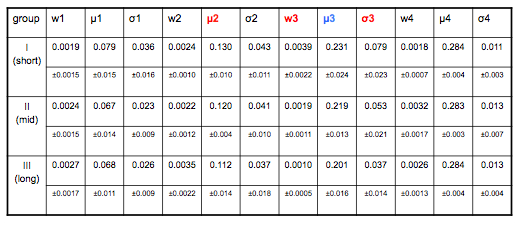
where w1, w2, w3, and w4 are weights, μ1, μ2, μ3, and μ4 are means, σ1, σ2, σ3, and σ4 are standard deviations for the 4 components respectively. Histogram data from individual cases was used to identify approximate threshold boundaries for each of the four components from Gaussian fitting. Spatial distribution of the 4 components within the tumor was localized accordingly.
Results
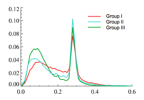
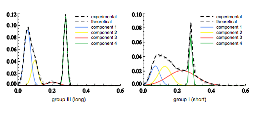
Visual examination of histogram of ve distributions showed apparent differences between the three survival groups. The average histogram from patients with long survival showed an almost bimodal distribution whereas patients with short survival appeared to show the same two peaks but with an increasing number of pixels representing intermediate values (Fig. 1). Following Gaussian fitting it can be seen that patients with short survival show an increasing proportion of pixels falling into the third Gaussian distribution (figure 2). The group average of the 12 estimated parameters (Eq. [2]) are given in Table 1. Among the 12 parameters, μ2 (P = 0.00015, R2 = 0.44), w3 (P = 0.0066, R2 = 0.26) and σ3 (P = 0.011, R2 = 0.23) correlated with survival. μ3 has a trend to correlate with survival (P = 0.072, R2 = 0.12). Fig 3 shows the spatial distribution of the 4 components within the tumor in a patient in Group III (the same patient as in the left panel of Fig. 2). The histogram was segmented to separate the 4 components, and the segment thresholds were used in the color-coding GBM ve maps for representing the spatial distribution of the 4 components in the tumor. However, due to the considerable overlapping between the blue and yellow components in this histogram, the separation of the blue and yellow distribution in the maps may not be accurate. Typically, component three tissue (red-coded) was identified within the spatial distribution of a larger area of component two (yellow-coded).Discussion
Gaussian fitting identified four separable components. Fitting parameters from the second and the third components of the Gaussian fits were the most predictive of overall survival. The increase in mean value of the 2nd Gaussian component (μ2, yellow-coded) and in the weight of the 3rd component (w3, red-coded) demonstrated strong correlation with overall survival.Conclusion
Histogram Analysis of ve identifies a tissue subpopulation which appears to have a very strong relationship to survival in GBM treated with standard Stupp therapy.Acknowledgements
No acknowledgement found.References
1. mills S, Plessis D, Pal P, et al. Mitotic Activity in Glioblastoma Correlates with Estimated Extravascular Extracellular Space Derived from Dynamic Contrast-Enhanced MR Imaging. AJNR Am J Neuroradiol. 2016; 37(5):811-7.
2. Li KL, Jackson A. New hybrid technique for accurate and reproducible quantitation of dynamic contrast-enhanced MRI data. Magn Reson Med 2003;50(6):1286 1295.
Figures