4149
Quantitative Magnetization Transfer Imaging of the Substantia Nigra in Parkinson’s Disease1Neurology, Vanderbilt University Medical Center, Nashville, TN, United States, 2Neuroradiology, Fondazione IRCCS Ca' Granda - Ospedale Maggiore Policlinico, Milan, Italy, 3FMRIB, University of Oxford, Oxford, United Kingdom, 4Vanderbilt University Institute of Imaging Science, Vanderbilt University, Nashville, TN, United States, 5Radiology and Radiological Sciences, Vanderbilt University, Nashville, TN, United States
Synopsis
Parkinson’s disease (PD) is characterized by the loss of pigmented dopaminergic neurons in the substantia nigra pars compacta (SNc). The aim of the study was to evaluate the feasibility of rapid magnetization pool size ratio (PSR) mapping as a subset of the magnetization transfer (MT) properties of the SNc in healthy subjects and patients with PD. These results demonstrated the feasibility of performing quantitative PSR mapping in human SN within reasonable scan times, and that PSR is likely the quantitative MT parameter most relevant for PD.
Purpose
Parkinson’s disease (PD) is characterized by the loss of neuromelanin-pigmented dopaminergic neurons in the substantia nigra pars compacta (SNc). Neuromelanin-sensitive MRI techniques 1 (NM-MRI), have shown notable contrast between the SNc and surrounding brain tissues, even in early stages of PD. Observations that magnetization transfer (MT) preparation of NM-MRI pulse sequences increases the SNc contrast 2 have led to the suggestion that MT may be used to characterize SNc properties in PD. Quantitative MT (qMT) techniques can be used to derive indices of tissue structure, 3,4 including: macromolecular-to-free pool size ratio $$$(PSR)$$$, the rate of MT exchange between pools $$$(k_{mf})$$$, and the longitudinal and transverse relaxation times for each pool $$$(T_{1,2}^{f,m})$$$, but are generally time consuming. The aim of this study was to apply qMT imaging to characterize the MT properties of the SN in healthy subjects and patients with PD, and to compare a rapid “single-point” measurement of $$$PSR$$$ with that of a “full” qMT model requiring twice the scan time.Methods
We examined 16 subjects with PD (13 males, 48-72 years old; disease duration: 2-10; Hoehn and Yahr: 1-3), and 8 age-matched healthy controls (HC) (3 males, 51-72 years old) using a 3T MRI scanner (Achieva, Philips Medical Systems, the Netherlands) with a 32-channel head coil. We performed two qMT protocols to allow comparison between: 1) a “full-fit” analysis based on low resolution images (acquired/reconstructed resolution=1.0×1.0/0.75×0.75 mm2) at eight offsets (Δω=1, 1.5, 2, 2.5, 8, 16, 32, 100 kHz) and two powers (αMT=600° and 900°) (acquisition time=8 min 5 s); and 2) a “single-point-fit” based on high-resolution images (acquired/reconstructed resolution =0.5×0.5/0.42×0.42 mm2) at Δω=2 kHz and 100 kHz, and αMT=900° (acquisition time=4 min 18 s). In all cases, data were acquired using a 3D MT-prepared SPGR sequence with a multi-shot EPI readout, EPI factor=5, TR/TE/α=47 ms/9 ms/10°, SENSE factor=2, and MT-weighting achieved using a 20-ms, single-lobed sinc-Gauss pulse. B0, B1 and T1 maps ($$$T_{1}^{obs}$$$) were acquired using 3D SPGR techniques. Finally, we acquired a NM-MRI scan (Figure 1c) consisting of a T1-weighted TSE sequence with the manufacturer’s default MT preparation pulses (TR/TE=670/12 ms, echo train length=4, acquired/reconstructed resolution=0.75×0.75/0.5×0.5 mm2, NSA=4, acquisition time=3 min 50 s). All scans were acquired as oblique axial slices (Figure 1) covering the midbrain, with a FOV=216×180×21 mm3, and slice thickness=3 mm.
Images were co-registered, and cropped to an area around the midbrain. MT-weighted images were normalized to the intensity of the reference image (Δω=100 kHz), and the nominal offset frequency and RF amplitudes were corrected using B0 and B1 maps, respectively. For the full-fit analysis, $$$PSR$$$, $$$k_{mf}$$$, $$$T_{2}^{f}$$$, and $$$T_{2}^{m}$$$ maps were generated using the model described in 3. $$$R_{1}^{f}$$$ values were derived from the $$$T_{1}^{obs}$$$ as described by 3. $$$PSR$$$ maps were also calculated according to the single-point fitting method described in 4,5. As fixed parameter values in the single-point qMT analysis, we used the median values of histograms of the $$$k_{mf}$$$, $$$R_{1}^{f}T_{2}^{f}$$$, and $$$T_{2}^{m}$$$ maps obtained in the full-fit analysis. Region of interest (ROI) in the SNc and the cerebral crus (CC) were defined in the NM-MRI images (Figure 1d) as described in 6. Differences between HC and PD groups were analyzed by means of the Wilcoxon test. Agreement between the full-fit and single-point methods was evaluated using Spearman correlation coefficient (ρ) and Bland–Altman plots.
Results
Full-fit $$$PSR$$$ maps (Figure 2a) provided clear differentiation between white and grey matter, and good visualization of the SNc. The $$$k_{mf}$$$, $$$R_{1}^{f}T_{2}^{f}$$$, and $$$T_{2}^{m}$$$ maps (Figure 2b-e) exhibited relatively constant values across tissues (median values: $$$k_{mf}=10.54 Hz$$$, $$$R_{1}^{f}T_{2}^{f}=0.0186$$$, $$$T_{2}^{m}=9.94 μs$$$) and did not provide notable contrast for the SNc. The single-point $$$PSR$$$ maps (Figure 3e-f) displayed higher contrast between SNc and CC than the full-fit $$$PSR$$$ maps (Figure 3c-d). We found a significant correlation between $$$PSR$$$ values obtained by the two methods (Figure 4a); there were no significant differences between the methods, but the single-point $$$PSR$$$ estimates presented lower variability than the full-fit results (Figure 4b). In the comparisons between HC and PD groups, we found significant differences only for the $$$PSR$$$ of the SNc (p<0.05). Table 1 summarizes the quantitative results from all analyses.Discussion and conclusion
The single-point approach provides high-resolution, lower-variability estimates of $$$PSR$$$ within clinically relevant scan times, thus providing a clinically applicable approach for qMT imaging in PD. Our initial results suggest an increased $$$PSR$$$ in the SNc in patients with PD, however, the limited number of subjects examined here necessitates cautious interpretation of these results as well as further validation through larger studies.Acknowledgements
This work was supported by a doctoral scholarship funded by Fondazione IRCCS Ca' Granda Ospedale Maggiore Policlinico di Milano (to PT), by grants DOD W81XWH-13-0073, NIH/NIBIB R21NS087465-01, NIH/NIBIB R01EY023240 01A1 and The National MS Society (to SAS), and by grants NIH/NINDS K23 NS080988, and NIH/NINDS 1R01NS097783-01 (to DOC).References
1. Sasaki M, Shibata E, Tohyama K, et al. Neuromelanin magnetic resonance imaging of locus ceruleus and substantia nigra in Parkinson’s disease. Neuroreport. 2006;17(11):1215-1218.
2. Schwarz ST, Bajaj N, Morgan PS, et al. Magnetisation Transfer contrast to enhance detection of neuromelanin loss at 3T in Parkinson’s disease. Proc. Intl. Soc. Mag. Reson. Med. 2013;21:2848.
3. Yarnykh VL, Yuan C. Cross-relaxation imaging reveals detailed anatomy of white matter fiber tracts in the human brain. Neuroimage. 2004;23(1):409-424.
4. Yarnykh VL. Fast macromolecular proton fraction mapping from a single off-resonance magnetization transfer measurement. Magn Reson Med. 2012;68(1):166-178.
5. Smith AK, Dortch RD, Dethrage LM, Smith SA. Rapid, high-resolution quantitative magnetization transfer MRI of the human spinal cord. Neuroimage. 2014;95:106-116.
6. Isaias IU, Trujillo P, Summers P, et al. Neuromelanin Imaging and Dopaminergic Loss in Parkinson’s Disease. Front Aging Neurosci. 2016;8:196.
Figures
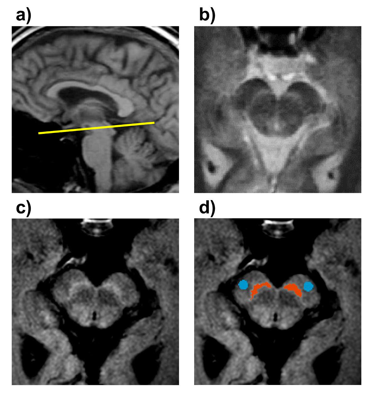
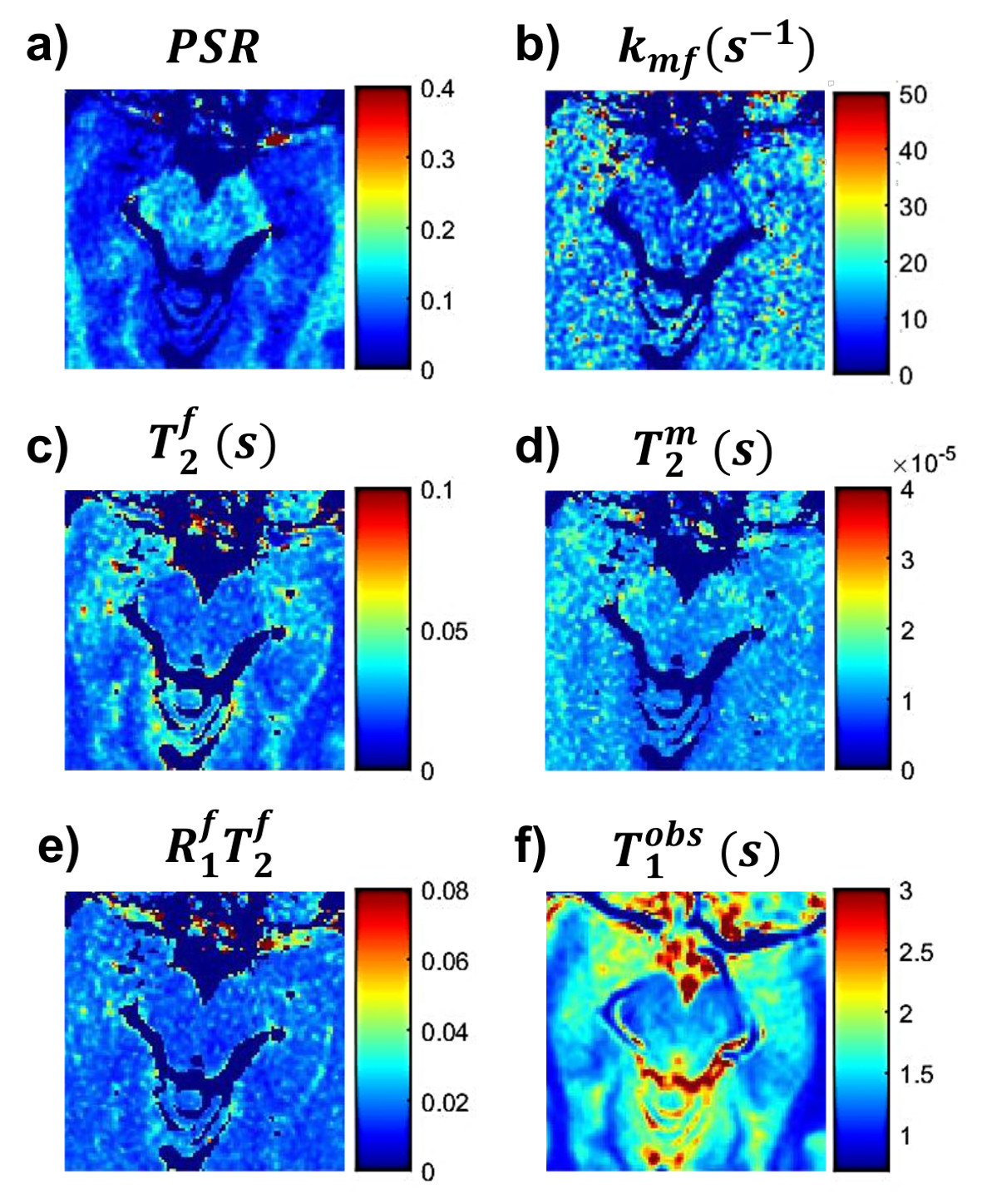
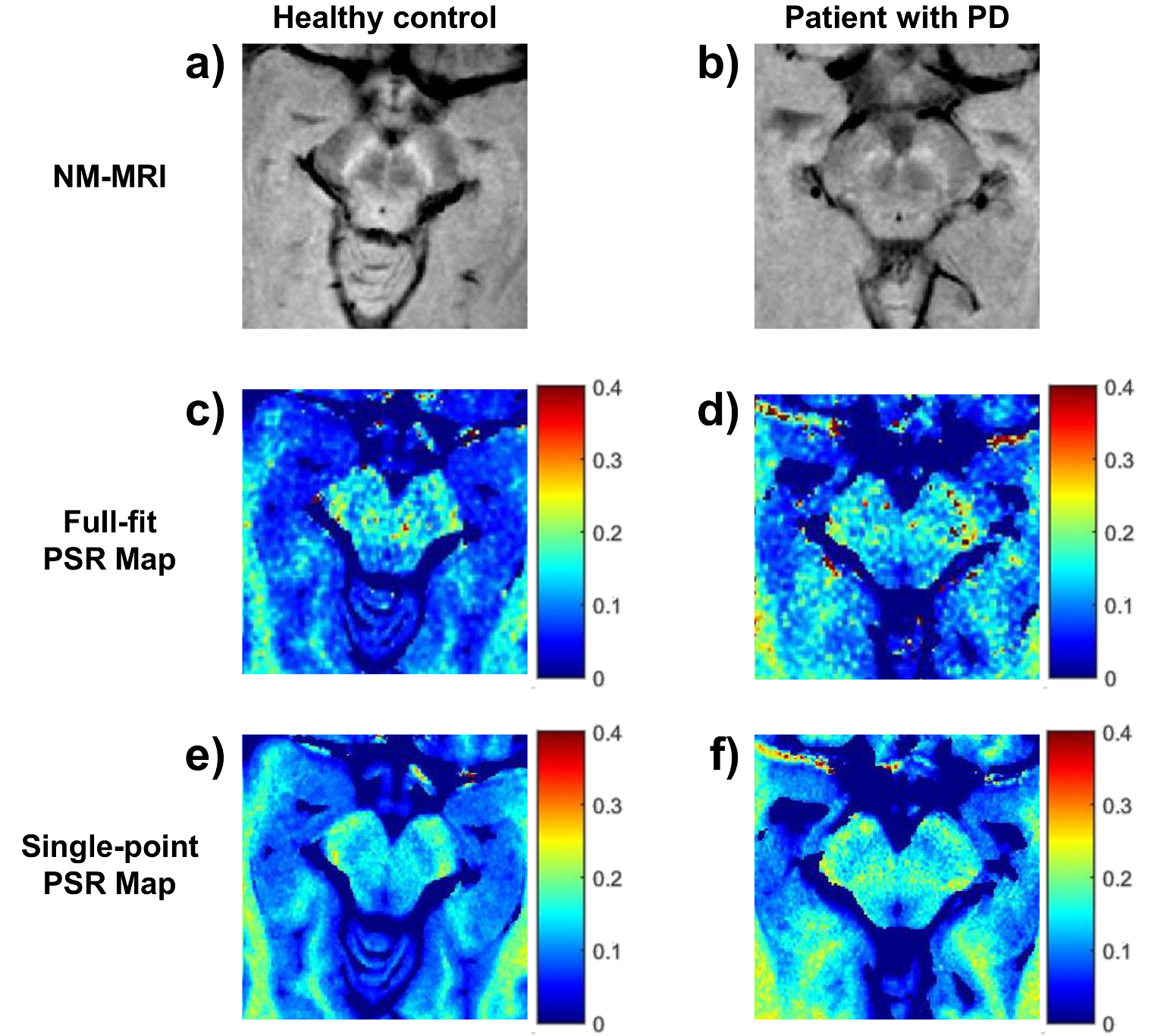
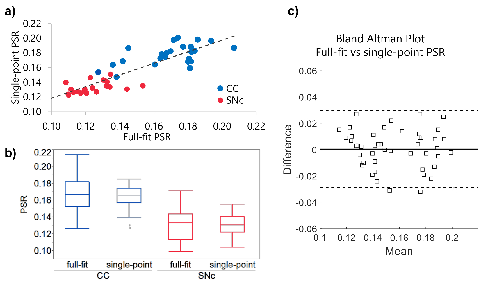
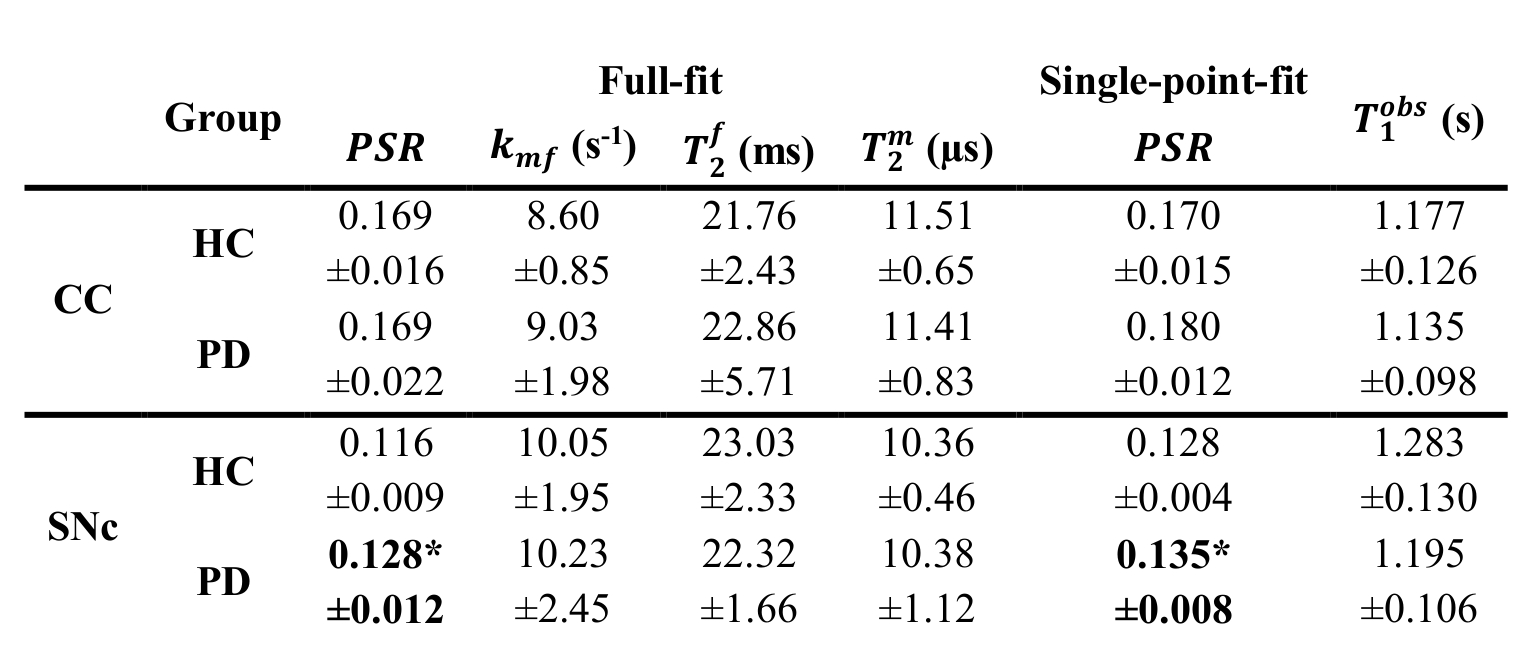
Table 1. Mean ± standard deviation of the quantitative estimates for the ROIs in the CC and SNc in the HC and PD groups. The first four columns show the quantitative indices obtained with the full-fit analysis, the fifth column shows the values for the $$$PSR$$$ estimated using the single-point approach, and the last column shows the $$$T_{1}^{obs}$$$ values. Only the $$$PSR$$$ values for the SNc (estimated using both approaches) were significantly different between HC and PD groups, with the PD patients having increased values.
* Significantly different between HC and PD (p<0.05).