4145

Distinct structural backbone-network in early Parkinson’s disease (PD) subjects: Insights from Parkinson’s Progressive Markers Initiative (PPMI) dataset

Virendra Mishra¹, Karthik Sreenivasan¹, Christopher Bird¹, Dietmar Cordes¹, and Ryan R Walsh¹

¹Cleveland Clinic Lou Ruvo Center for Brain Health, Las Vegas, NV, United States

Synopsis

In vivo imaging that reliably captures the impact of the spreading pathology of Parkinson’s disease (PD), including its impact on both white and gray matter, remains elusive. In this study, we applied graph-theoretical techniques to multi-site diffusion-MRI data from a cohort of early PD-subjects in Parkinson’s Progressive Markers Initiative (PPMI) database. A distinctive structural backbone-network was revealed in early PD-subjects without any a-priori assumptions involving cortical and subcortical regions that are known to be involved in various stages of PD, including early PD (Olfactory-cortex, globus-pallidum, and striatum). Our study opens new avenues to understanding progression of PD from a graph-theoretical approach.

Introduction

The pathologic development of Parkinson’s disease (PD) appears to be related to the spread of abnormal synuclein in a largely caudal-rostral direction in the CNS^1–3. In vivo imaging that captures the impact of this spreading pathology on both white and gray matter remains elusive^4,5. Graph-theoretical approaches have the ability to characterize connectivity at both global and local levels⁶. Structural backbone network with graph-theoretical methods have been shown to exist in healthy controls⁷ but whether there is a shift in this network in early PD has not been investigated to the best of our knowledge. Hence, we applied graph-theoretical approaches to diffusion-MRI data from the Parkinson’s Progressive Markers Initiative (PPMI) database⁸ and characterized backbone structural networks which may in turn help differentiate controls from PD early in the disease.

Methods

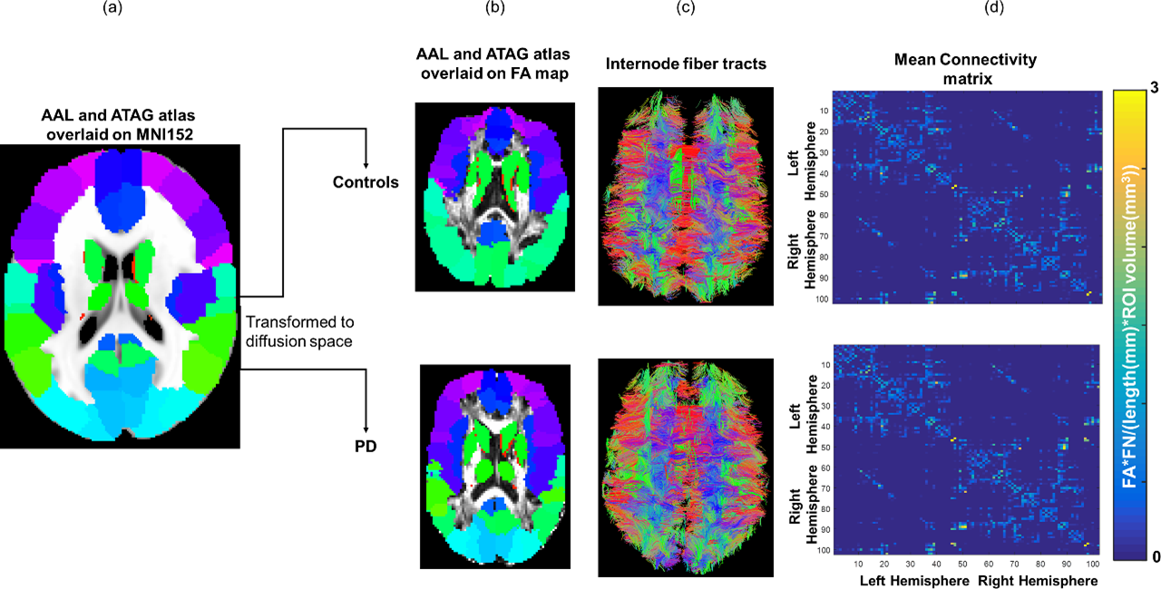
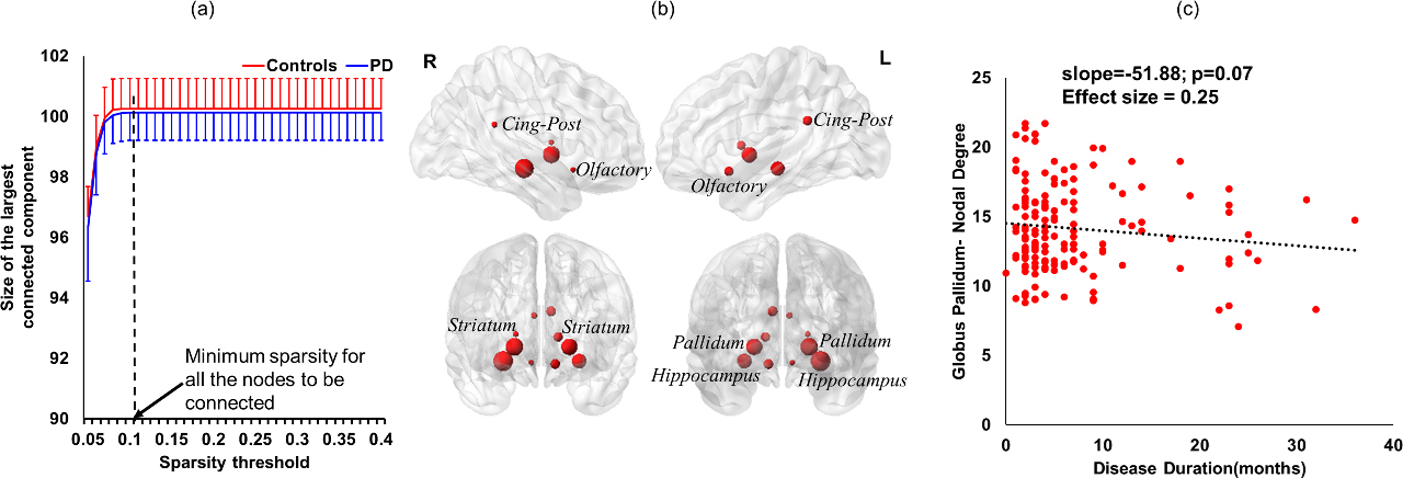
Subjects: Diffusion-MRI and T1-weighted MRI data from 69 (24 female) healthy controls (age: 60.61±10.61years, years of education (YOE): 15.61±3.07) and 151 (53 female) early PD-subjects (age: 61.03±9.23years, YOE: 15.14±2.95, total MDS-UPDRS: 30.81±13.03; disease duration: 7±7.14months) were derived from PPMI for this study. Imaging parameters are described in detail at http://www.ppmi-info.org/⁸. Only data from 3T Siemens scanners with the first visit were used to ensure uniformity of diffusion data. Network construction: Two different atlases, AAL (mainly cortical)⁹, and ATAG (subcortical)¹⁰ in MNI space, were used to generate 102 nodes (90 AAL-nodes and 12 ATAG-nodes) of the network. T1-weighted MNI152 brain was normalized to each subject’s native diffusion space and the resultant transformation matrix was applied to both the atlases to get the nodes in subject’s native space. Whole brain tractography was performed using diffusion toolkit (http://www.trackvis.org/dtk/)¹¹. The nodes were expanded by four voxels¹² and only those fiber-tracts that had ends in either nodes were retained. Fibers smaller than 6mm and internode connectivity with less than 10 fibers were filtered from any further analysis. Each internode connection (edge) was weighted by the product of the number of fibers and average FA of the fibers connecting the two nodes and normalized by the product of average length of the fibers and summation of volume of the two nodes. Backbone-network: Nonparametric sign test, Bonferroni corrected p<0.05, was performed within each group and those edges that had a significantly greater chance to be present in each subject within each group were retained and characterized as a structural backbone-network of the group⁷. Graph-theoretical measures: Degree, betweenness-centrality (bc) and modularity measures were computed using GRETNA¹³ to characterize the location of the hubs within each group. Various sparsity thresholds (5-40%, step=1%) were used to identify the minimum sparsity at which the network is fully connected. Nodes where normalized-bc were greater than (mean(normalized-bc)+1.5*standard-deviation(normalized-bc)) at the chosen sparsity level were identified as hubs¹⁴. Statistical analysis: A linear regression between nodal degree and disease duration was performed for two most important hubs, as identified by bc, after controlling for age, gender, and years of education.

Results

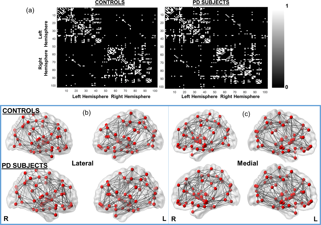
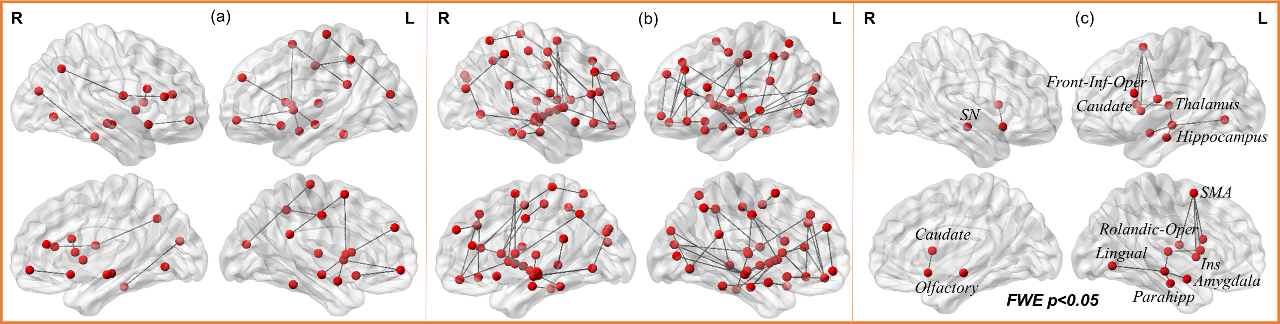
As expected, most of the cortical-subcortical fibers (Fig.1(c)) were retained (representative healthy control (top-row) and PD-subject (bottom-row)) as internode fibers. The mean connectivity matrix (Fig.1(d)) do not reveal any qualitative differences between the groups. Binarized backbone structural connectivity matrix in controls (Fig.2(a), left-row) and PD (Fig.2(a), right-row) had a sparsity of 9% (98 nodes) and 10% (100 nodes) contributing to the backbone-network, respectively. Fig.2(b) visualizes the backbone-network for both the groups. There were 19 paths identified to be only present in controls (Fig.3(a)) mainly comprising of supplementary-motor area, striatum, cingulum, angular gyrus, caudate, hippocampus, and thalamus. There were 90 paths exclusively present in PD (Fig.3(b)) involving all the subcortical regions along with insula, parahippocampal gyrus, and entire cingulum. Network-based-statistics revealed 14 paths (Fig.3(c)) where controls had a significantly greater (pcorrected<0.05) anatomical connectivity comprising of medial temporal lobe and subcortical regions. Bilateral hippocampus, globus-pallidus (GP), striatum, olfactory cortex (OC), and posterior-cingulum were identified as hubs in both the groups at a sparsity of 10% (Fig.4 (a) and (b)). There was a trend (p=0.07) of negative association of right GP degree with disease duration (Fig.4(c)).

Discussion

Without any a-priori assumptions, our study shows a distinctive backbone-network in early PD involving cortical and subcortical regions that are known to be involved in various stages of PD, including early PD (OC, GP, striatum)^1,2. We are currently investigating shift in this backbone-network or other network measures can be used to predict disease progression and severity.

Conclusion

Graph-theoretical study of early PD subjects revealed a structural backbone-network that is different from controls and consistent with post-mortem studies, thereby opening new avenues to understanding progression of PD.

Acknowledgements

The study was supported in parts by National Institute of General Medical Sciences (grant: P20GM109025) and the Elaine.P.Wynn and family foundation.

References

1. Braak H, Del Tredici K, Rub U, de Vos RAI, Jansen Steur ENH, Braak E. Staging of brain pathology related to sporadic Parkinson’s disease. Neurobiol Aging 2003; 24: 197–211.

2. Braak H, Bohl JR, Muller CM, Rub U, de Vos RAI, Del Tredici K. Stanley Fahn Lecture 2005: The staging procedure for the inclusion body pathology associated with sporadic Parkinson’s disease reconsidered. Mov Disord 2006; 21: 2042–51.

3. Goedert M, Spillantini MG, Del Tredici K, Braak H. 100 years of Lewy pathology. Nat Rev Neurol 2013; 9: 13–24.

4. Hall JM, Ehgoetz Martens KA, Walton CC, et al. Diffusion alterations associated with Parkinson’s disease symptomatology: A review of the literature. Parkinsonism Relat Disord 2016; published online Sept. DOI:10.1016/j.parkreldis.2016.09.026.

5. Pyatigorskaya N, Gallea C, Garcia-Lorenzo D, Vidailhet M, Lehericy S. A review of the use of magnetic resonance imaging in Parkinson’s disease. Ther Adv Neurol Disord 2014; 7: 206–20.

6. Bullmore E, Sporns O. Complex brain networks: graph theoretical analysis of structural and functional systems. Nat Rev Neurosci 2009; 10: 186–98.

7. Gong G, He Y, Concha L, et al. Mapping Anatomical Connectivity Patterns of Human Cerebral Cortex Using In Vivo Diffusion Tensor Imaging Tractography. Cereb. Cortex (New York, NY). 2009; 19: 524–36.

8. www.ppmi-info.org.

9. Tzourio-Mazoyer N, Landeau B, Papathanassiou D, et al. Automated anatomical labeling of activations in SPM using a macroscopic anatomical parcellation of the MNI MRI single-subject brain. Neuroimage 2002; 15: 273–89.

10. Keuken MC, Bazin P-L, Crown L, et al. Quantifying inter-individual anatomical variability in the subcortex using 7 T structural MRI. Neuroimage 2014; 94: 40–6.

11. Wang R, Wedeen VJ. TrackVis.org. In: Proc Intl Soc Mag Reson Med. 2007: 3720.

12. Jeon T, Mishra V, Huang H. Effects of cortical regions of interests on tractography and brain connectivity quantification. In: Proc Intl Soc Mag Reson Med. 2016: 2063.

13. Wang J, Wang X, Xia M, Liao X, Evans A, He Y. GRETNA: a graph theoretical network analysis toolbox for imaging connectomics. Front Hum Neurosci 2015; 9: 386.

14. He Y, Chen Z, Evans A. Structural insights into aberrant topological patterns of large-scale cortical networks in Alzheimer’s disease. J Neurosci 2008; 28: 4756–66.

Figures

Fig.1: (a) AAL (mainly cortical) and ATAG (sub-cortical) nodes are overlaid on MNI brain (b) Both AAL and ATAG atlases were transformed to subject’s native diffusion space and overlaid on a representative subject’s fractional anisotropy (FA) map. (c) Cortical-subcortical fibers retained as the internode fibers that were used to build the connectivity matrix. (d) Mean connectivity matrix for controls and early PD-subjects. Top and bottom row represent data from controls and PD-subjects respectively. Color-bar represents the connectivity strength in the mean connectivity matrix.

Fig.1: (a) Binarized structural backbone network for controls (left) and PD-subjects (right). The structural connectivity matrix was visualized on MNI brain. Both lateral (b) and medial (c) views are shown. Red circle represents the location of the nodes where the backbone network exists. The line connecting the nodes represents the connections between the nodes. The top and bottom row in (b) and (c) visualizes the backbone network in controls and PD-subjects respectively.

Fig.3: (a) The nodes and edges that were exclusively present in the backbone network of controls (a) and PD-subjects (b) are visualized on MNI brain. (c) The paths that were significantly greater in controls were extracted through network based statistic. Red circle represents the approximate location of the nodes. The line connecting the nodes represents the connections between the nodes. FWE: Familywise error corrected

Fig.4:(a) Size of the largest connected component at different sparsity threshold is plotted for both controls(red) and PD-subjects(blue). The error bar represent the standard deviation for each group at each threshold. The dashed line represents the threshold where both the groups have the entire network connected.(b) Red circle represents the hubs for both the groups. The size of the circle represent the difference in betweenness-centrality of controls and PD-subjects.(c) Nodal degree was extracted for every PD-subject in right Globus-Pallidum hub(2nd-most-important hub) and regressed against disease duration. Each scatter represent mean nodal degree at sparsity threshold of 10% for every PD-subject.

Proc. Intl. Soc. Mag. Reson. Med. 25 (2017)

4145