4055
Manifold valued statistical models for longitudinal analysis of MRI data1Waisman Center, University of Wisconsin-Madison, Madison, WI, United States, 2Computer Sciences, University of Wisconsin-Madison, 3Psychology and Psychiatry, University of Wisconsin-Madison, 4Medical Physics and Psychiatry, University of Wisconsin-Madison, 5Medicine, University of Wisconsin-Madison, 6Biostatistics and Computer Sciences, University of Wisconsin-Madison
Synopsis
This work presents novel statistical image analysis methods to characterize complex morphological brain changes using MRI data. Specifically, our procedure utilizes the fundamental representations of "longitudinal change" -- voxel-wise Jacobian matrices obtained from image registration. Currently their univariate summaries (for example determinants) are ubiquitously used in neuroimaging studies. Operating directly with representations of Jacobians namely Cauchy deformation tensors, which are elements of an abstract mathematical manifold of symmetric positive definite matrices, yields promising improvements in statistical power in detecting subtle but statistically significant effects. The key technical contributions are computational algorithms for estimating multivariate general linear models with manifold-valued response variables.
Introduction
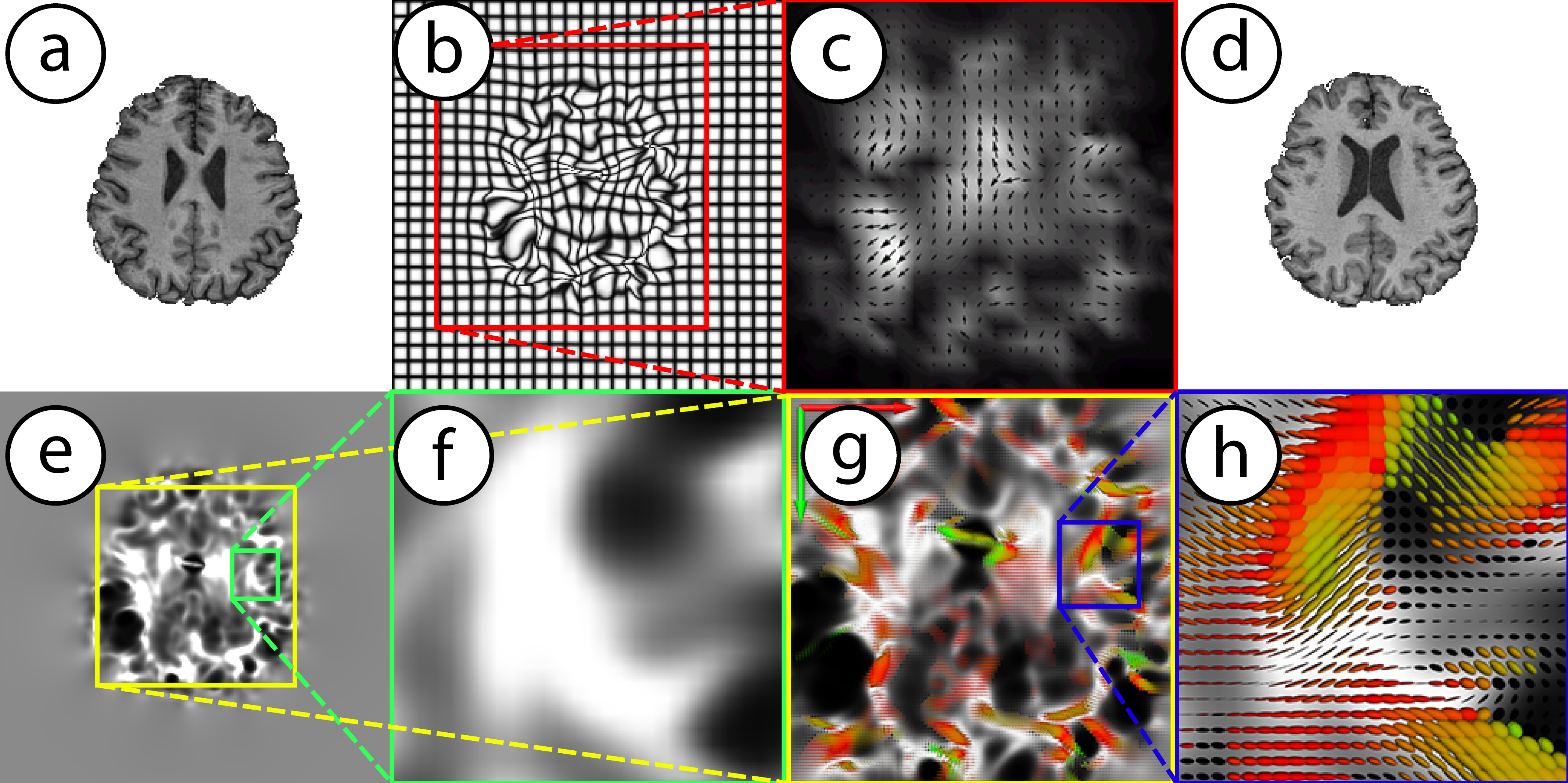
Longitudinal changes of the brain structure can be estimated using registration of $$$T_1$$$-weighted MRI data. The Jacobian $$$\left(J\right)$$$ of the deformations provides information about the volumetric as well as shape specific changes. The determinant of the Jacobian $$$\left(|J|\right)$$$ represents relative volume change between time points ($$$|J|<1$$$: volume loss, $$$|J|>1$$$: volume gain). Using general linear model regression analysis one can then identify interesting associations between brain volumetric changes and clinical covariates. But summarizing the Jacobian into a determinant represents the subject-wise deformation at a much coarser scale, potentially decreasing statistical power in studies where the effect sizes are already small. Instead, as shown in Fig. 1 one could perform analysis using the Cauchy deformation tensor (CDT) defined as $$$\sqrt{J^TJ}$$$. CDTs are $$$3\times 3$$$ symmetric positive definite (SPD) matrices which form an abstract mathematical manifold1-7. The key technical difficulty in performing regression analysis using CDTs is that for curved spaces such as SPD manifolds, the standard arithmetic operations like addition, subtraction and multiplication cannot be applied directly. These operations must be re-derived using concepts from differential geometry for each specific statistical model we wish to run on our morphometric maps represented by CDT images. Specialized computational optimization methods for estimating the models are needed. In summary, while CDTs are promising extension to $$$|J|$$$ for longitudinal morphometric analysis, the associated analysis methods pose unique challenges. Our work presents a computational framework to perform manifold valued general linear model (MGLM) regression analysis with multiple covariates.Methods
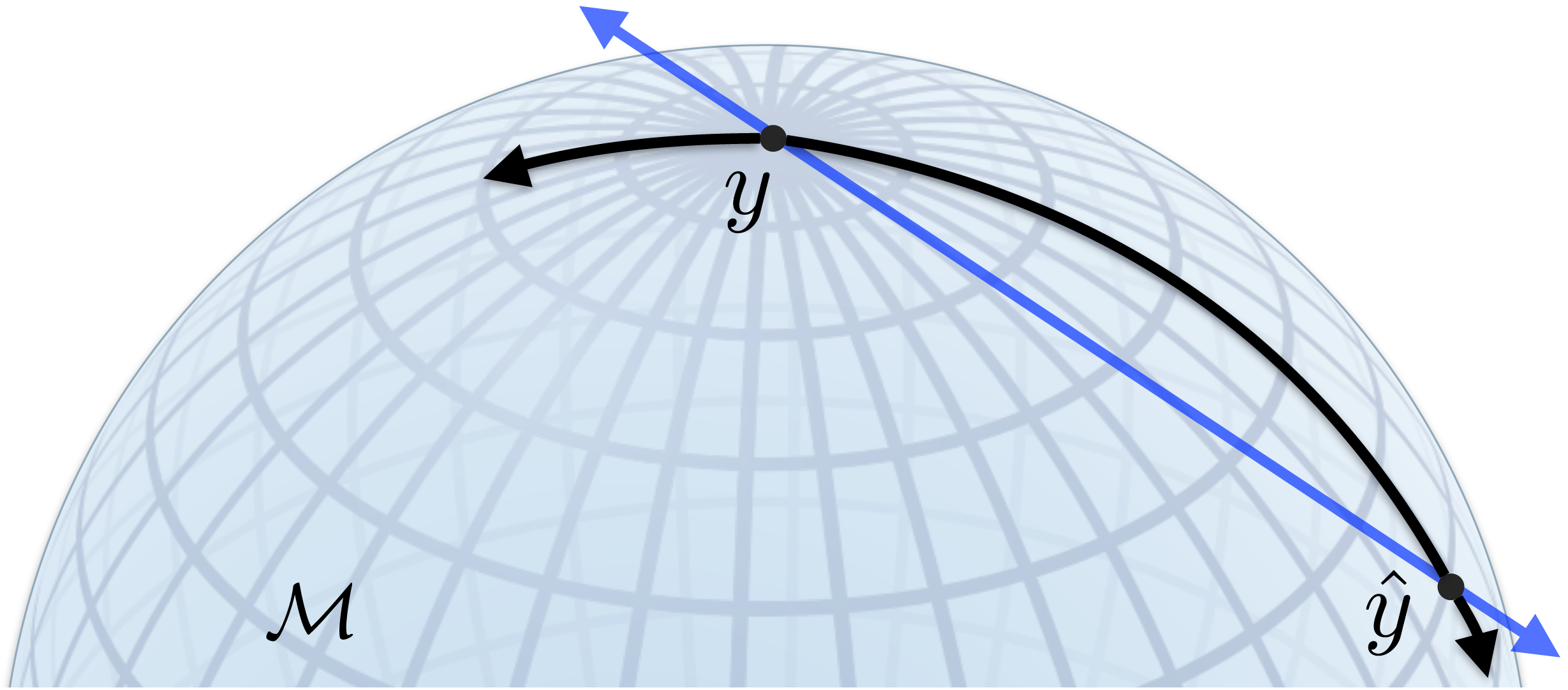
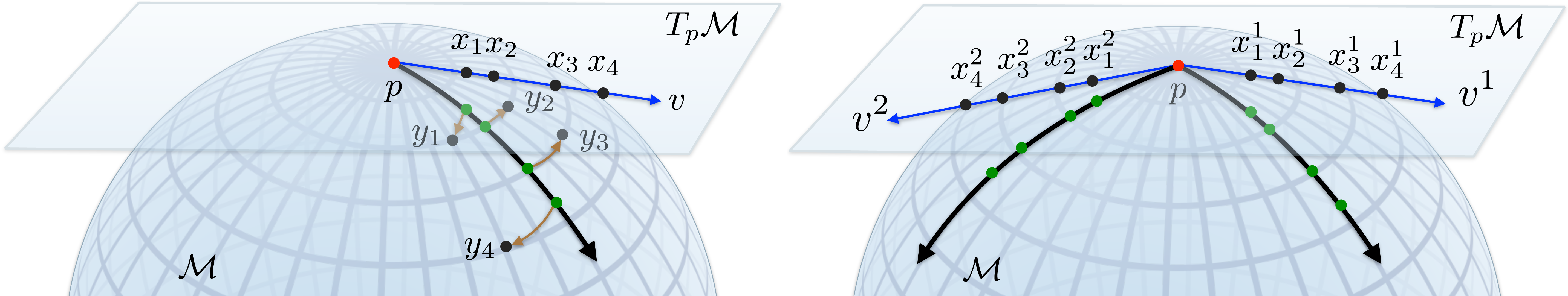
Let us consider a standard voxel-wise analysis setup. A general linear model (GLM) identifies associations between covariates and the measurements at each voxel. For each voxel $$$i$$$, we solve $$$y_i=\alpha+\mathbf{\beta}^T\mathbf{x}_i+\varepsilon_i$$$, for $$$\alpha$$$, the $$$y$$$-intercept and $$$\mathbf{\beta}$$$, a $$$p$$$-dimensional coefficient vector for the covariates $$$\mathbf{x}_i=\{x_i^{1},x_i^{2},\ldots,x_i^{p}\}$$$. $$$\varepsilon_i$$$ is the error in the voxel measurement $$$y_i$$$. Using data from $$$N\geq (p+1)$$$ subjects, the coefficients $$$\alpha$$$ and $$$\beta$$$ can be estimated by minimizing the residual $$$\displaystyle\sum_{j=1}^N\left(y_i^j-\alpha-\mathbf{\beta}^T\mathbf{x}_i^j\right)^2$$$. When the response is a CDT (SPD matrix) we cannot directly perform an element-by-element subtraction of the matrices for computing residuals1,6,7. To see this, consider a manifold visualized in Fig. 2 in the context of the subtraction operation. The residual (or distance) between the measurement $$$y$$$ and the model prediction $$$\hat{y}$$$ should in principle be the shortest geodesic curve (black) connecting $$$y$$$ and $$$\hat{y}$$$ that lies on the manifold. A direct element-by-element subtraction estimates the length of the straight line (blue) that lies in the ambient space and not entirely on the manifold. This can be a poor approximation when the curvature of the manifold is high. Such approximations may result in reduction of power for detecting statistical associations between $$$\mathbf{x}$$$ and $$$y$$$. Hence the distance $$$(y-\hat{y})$$$ should be computed by an operation that measures the length of the shortest curve connecting these two matrices along the manifold.For simplicity, we present the main ideas in our algorithms for computing residuals using a single covariate $$$(p=1)$$$ MGLM. There are two main pieces in minimizing the residual. (1) $$$\alpha$$$ which corresponds to a distinct unknown point on the manifold serves as an “offset”. This offset will be used to define a tangent space – a plane locally tangent to the manifold (Fig. 3). (2) The coefficient $$$\beta$$$, in our formulation, corresponds to a vector $$$v$$$ in the tangent space. It turns out that the tangent vector $$$v$$$ precisely corresponds to a “geodesic curve” on the manifold (shown in black in Fig. 3). Thus we can parameterize geodesic curves via tangent vectors. Then using concepts from differential geometry8-12, we can compute the primary quantity of interest (residual), directly on the manifold. The GLM estimation procedure then reduces to searching through possible values of the offset and the tangent vector such that residual is as small as possible. The technical details when $$$p>1$$$ (Fig. 3, right) are more complicated but conceptually similar to the $$$p=1$$$ case. Since statistics using manifold-valued data do not satisfy many of the standard parametric-distributional assumptions, $$$p$$$-values can be obtained using permutation testing.
Results
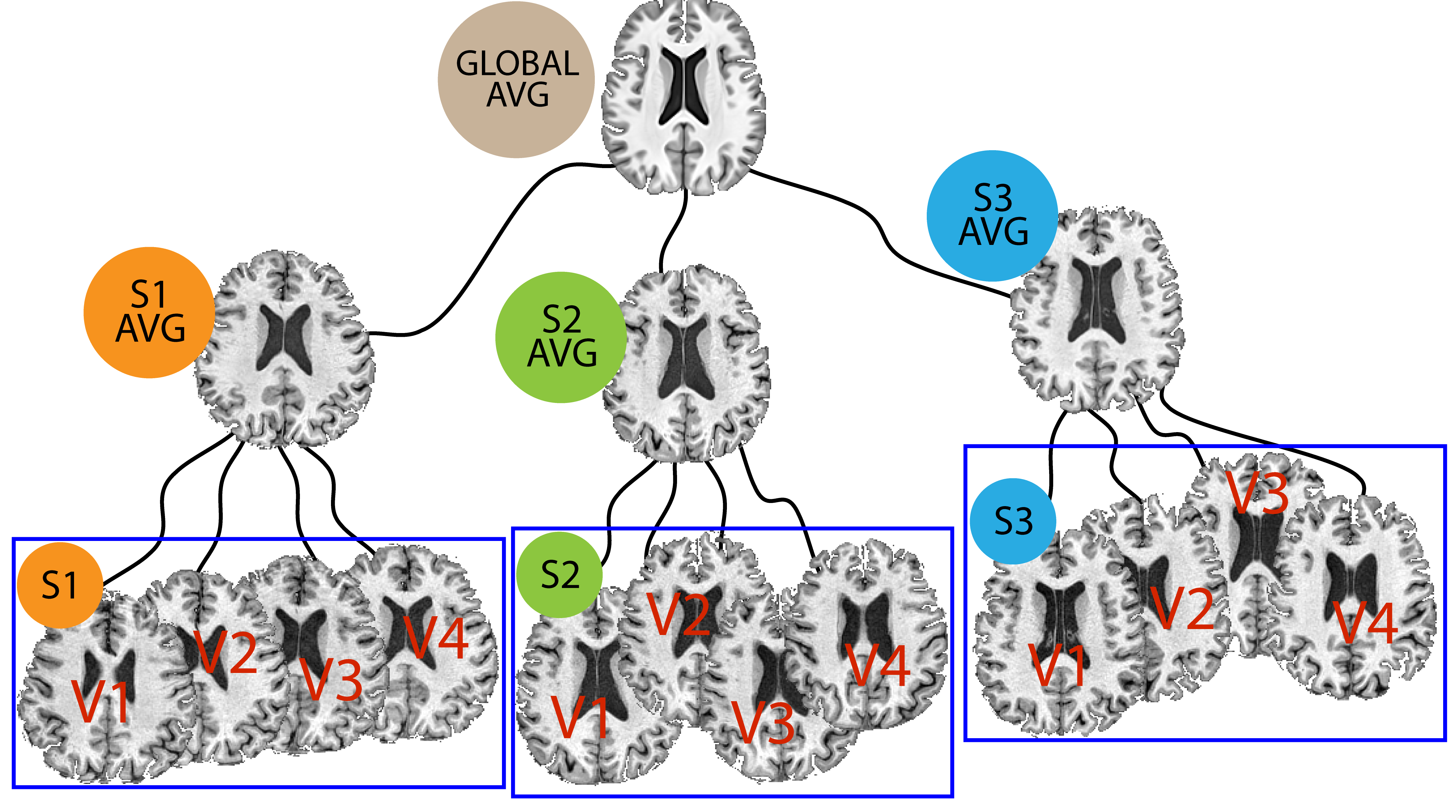
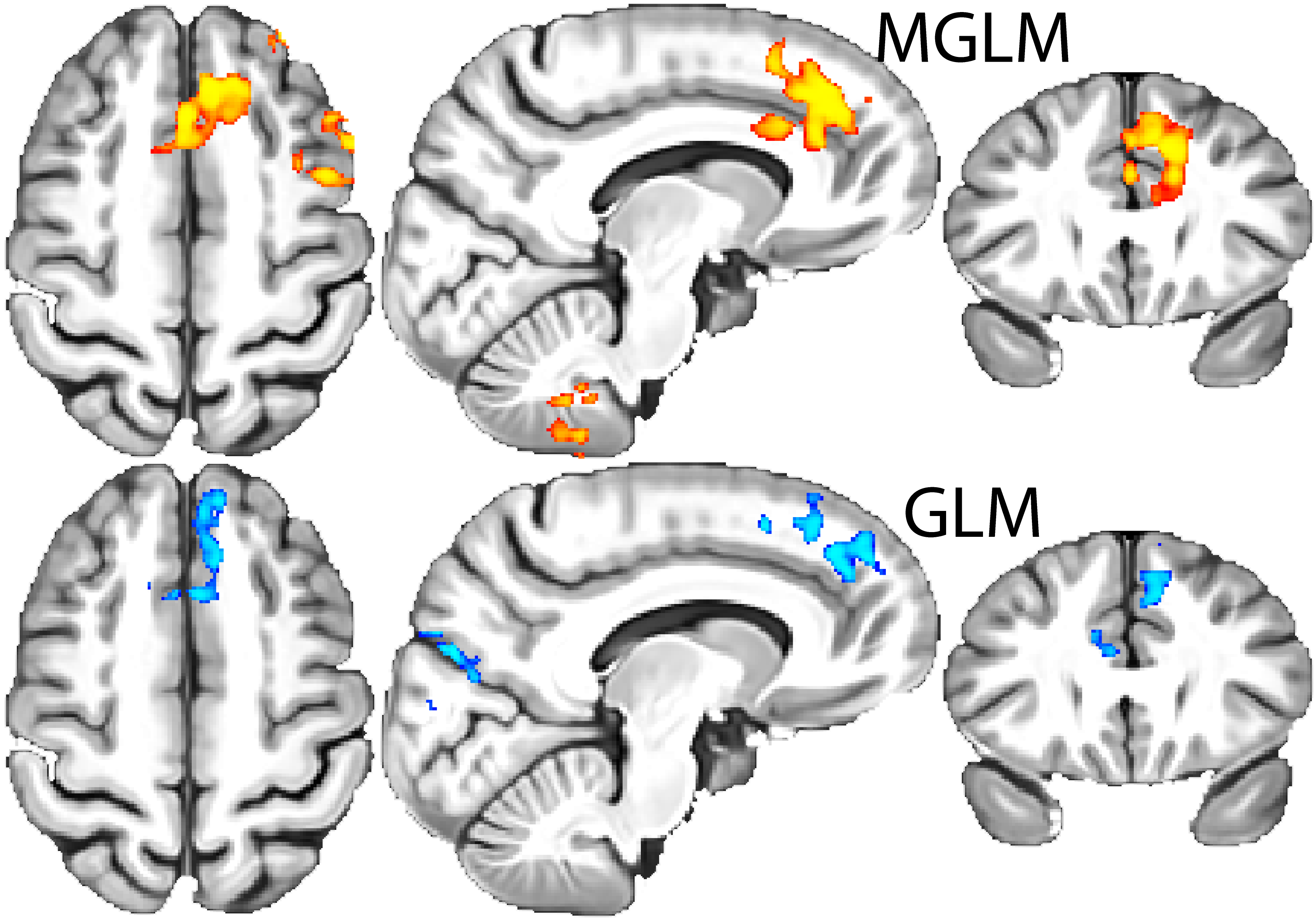
The longitudinal population average template image necessary for unbiased voxelwise analysis is shown in Fig. 4. Statistical analysis was performed using data from a pre-clinical Alzheimer's disease study to identify associations between CDTs and amyloid burden. Age and sex were control covariates (hence $$$p=3$$$). Fig. 5 summarizes the results comparing to those obtained from the analysis using Jacobian determinants.Discussion and conclusion
The $$$p$$$-values of statistical associations using CDTs are lower than those using $$$|J|$$$. These improvements provide promising evidence that computational algorithms for manifold-valued statistical analysis can be effective for longitudinal analysis of MRI data.Acknowledgements
This work was supported in part by NIH grants R01-EB02883, UL1RR025011, AG0033514, AG040396, NSF 1252725 and NIH P30-HD003352.References
1. Fletcher P. and Joshi S. Principal geodesic analysis on symmetric spaces: Statistics of diffusion tensors. Computer Vision and Mathematical Methods in Medical and Biomedical Image Analysis, ed: Springer, 2004, pp. 87-98.
2. Lenglet C., Rousson M., Deriche R. and Faugeras O. Statistics on the manifold of multivariate normal distributions: Theory and application to diffusion tensor MRI processing. Journal of Mathematical Imaging and Vision, 2006, vol. 25, pp. 423-444.
3. Friedrichs K. Symmetric positive linear differential equations. Communications on Pure and Applied Mathematics, 1958, vol. 11, pp. 333-418.
4. Bhatia R. and Holbrook J. Riemannian geometry and matrix geometric means. Linear Algebra and its applications, 2006. vol. 413, pp. 594-618.
5. Arsigny V., Fillard P., Pennec X. and N. Ayache. Geometric means in a novel vector space structure on symmetric positive-definite matrices. SIAM Journal on Matrix Analysis and Applications, 2007, vol. 29, pp. 328-347.
6. Jayasumana S., Hartley R., Salzmann M., Li H. and Harandi M. Kernel methods on the Riemannian manifold of symmetric positive definite matrices. Computer Vision and Pattern Recognition (CVPR), 2013, pp. 73-80.
7. Moakher M. A differential geometric approach to the geometric mean of symmetric positive-definite matrices. SIAM Journal on Matrix Analysis and Applications, 2005, vol. 26, pp. 735-747.
8. Helgason S. Differential geometry, Lie groups, and symmetric spaces. Academic press, 1979, vol. 80.
9. Eguchi T., Gilkey P. and Hanson A. Gravitation, gauge theories and differential geometry. Physics reports, 1980, vol. 66, pp. 213-393.
10. Do Carmo M. Differential geometry of curves and surfaces. Prentice-hall Englewood Cliffs, 1976, vol. 2.
11. Kobayashi S. and Nomizu K. Foundations of differential geometry. Vol 1: New York, 1963.
12. Spivak M. A comprehensive introduction to differential geometry. vol. 2, IV[A] Boston, Mass., 1970.
Figures