4041
Multi-compartment T2 relaxometry Model using Gamma Distribution representations: A framework for Quantitative Estimation of Brain Tissue Microstructures.1VisAGeS, IRISA U746, Universite de Rennes-1, Rennes, France, 2VisAGeS Inserm U746, IRISA, Inria, Rennes, France, 3Boston Children’s Hospital, Boston, MA, United States, 4VisAGeS, INRIA/IRISA, Inserm U746, CNRS, Rennes, France
Synopsis
Advanced MRI techniques (e.g. – d-MRI, MT, relaxometry etc.) can provide quantitative information of brain tissues. Image voxels are often heterogeneous in terms of microstructure information due to physical limitations and imaging resolution. Quantitative assessment of the brain tissue microstructure can provide valuable insights into neurodegenerative diseases (e.g. - Multiple Sclerosis). In this work, we propose a multi-compartment model for T2-Relaxometry to obtain brain microstructure information in a quantitative framework. The proposed method allows simultaneous estimation of the model parameters.
Purpose
Propose a method to obtain a quantitative estimation of brain tissue microstructure information from T2 relaxometry.Background
Damage to Myelin is a critical preliminary stage in neurodegenerative diseases such as Multiple Sclerosis (MS). Demyelination is usually followed by loss of axons and accumulation of fluids due to inflammation. Although demyelination may be reversible, loss of axons is irreversible. Hence, quantifying the tissue microstructures can provide information on the diseases status.
MRI image voxels are heterogeneous in terms of tissue microstructures due to imaging resolution constraints. This presents a challenge in having a quantitative assessment of critical structures. Myelin is a highly dehydrated structure leading to short T2 relaxation times (10-55ms)1,2. The CSF and fluid accumulated due to inflammation have high T2 relaxation times (till$$$\,$$$~2sec). T2 relaxation times for water contained in other cellular structures (as axons, etc.) are in the order of$$$\,$$$~80ms. Advanced MRI techniques as multi-echo T2 relaxometry sequences can be used to capture this distinguishing characteristic of the compartments. In this work we propose a signal model to estimate water fractions corresponding to: (1) Myelin, (2) Cellular structures as axons, (3) Free$$$\,$$$fluids in a voxel obtained from a T2 relaxometry sequence such as turbo Spin Echo (TurboSE) Sequence.
Method
Since the data is acquired using a multi-contrast TurboSE sequence, the echo decay is not purely exponential, but rather derived from methods as EPG3. T2$$$\,$$$signal space is modeled as a weighted mixture of probability distributions corresponding to the compartments. Voxel signal,$$$\;s(t_i),\;$$$at$$$\,i$$$-th echo$$$\,(TE=t_i)\,$$$is modeled as:
$$s\left(t_i\right)={M_0}\;\sum_{j=1}^{3}{w_j}{\displaystyle\int\limits_{T_2}}{\small{{f_j}\left(T_{2}\right)\;EPG\left(T_{2},\triangle{TE},i,T_1,B_1\right)\;dT_2}}$$
where,$$$\;M_0\;$$$is a constant.$$$\;j=\lbrace1,2,3\rbrace\,$$$represent$$$\,$$$compartments;$$$\,w_j$$$:$$$\,$$$Weight of each compartment;$$$\,\mathrm{B_1}$$$:$$$\,$$$Field inhomogeneity.$$$\;f_j(T_2;k_j,\theta_j)$$$:$$$\,$$$Gamma PDF describing each compartment in T2$$$\,$$$space. Gamma PDF was chosen observing its properties as non-negativity,skewness.$$$\;\lbrace{k_j,\theta_j}\rbrace_{j=1}^{3}\;$$$are the shape and scale parameters respectively of the Gamma PDF. Hence the cost function optimized for each voxel data series is:
$$\min_{\mathbf{K,\Theta,C,}B_1}\sum_{i=1}^{m}\left({y_i-\sum_{j=1}^{3}c_j\lambda_j(t_i;k_j,\theta_j,B_1)}\right)\;=\;\min_{\mathbf{K,\Theta,c,}B_1}\parallel{\mathbf{Y}-\mathbf{\Lambda}({\small{\mathbf{K,\Theta,}B_1}})\mathbf{C}}\parallel_{2}^{2}$$
where$$$\;\mathrm{Y}\in\mathbb{R}^m\;$$$is the observed signal and$$$\;m=$$$number of echoes.$$$\:\mathrm{K}=\lbrace{k_i}\rbrace_{i=1}^{3}\,$$$and$$$\:{\Theta}=\lbrace{\theta_i}\rbrace_{i=1}^{3}$$$:$$$\,$$$Shape and Scale parameter vectors respectively.$$$\:{C}\in\mathbb{R}^3\,$$$is a vector of scaled weights:$$$\;c_j=M_0w_j\;$$$from which the weights are obtained as:$$$\;w_j=c_j/\sum_i{c_i}$$$. $$$\Lambda\in\mathbb{R}^{m\times3}$$$ whose elements are formulated as:
$$\mathbf{\Lambda}_{i,j}=\lambda_j(t_i;k_j,\theta_j,B_1)={\displaystyle\int\limits_{T_2}}{\small{\frac{1}{\Gamma(k_j)\theta_{j}^{k_j-1}}T_{2}^{k_j-1}\exp\left(\frac{-T_2}{\theta_j}\right)\;EPG\left(T_2,\triangle{TE},i,T_1,B_1\right)\;dT_2}}$$ Parameters$$$\;\lbrace{\mathrm{K},\Theta,C}\rbrace\;$$$are estimated in a single step.$$$\;\mathrm{B_1}\;$$$is computed by a gradient free optimizer (BOBBYQA6) as it does not have any closed form solution3. We perform$$$\,\mathrm{c}\,$$$and$$$\,\mathrm{B_1}\,$$$optimization alternatively till convergence is obtained in desired error limit.
Since the variables to be estimated are linearly separable, we follow VARPRO approach4. Cost$$$\,$$$function is re-evaluated as:$$$\;\min_{{\mathrm{K},\Theta}}\parallel{{\mathrm{P}^{\bot}_{\Lambda}\mathrm{Y}}}\parallel_{2}^{2}\;$$$where$$$\;\mathrm{{{P}^{\bot}_{\Lambda}}={I}-{\Lambda\Lambda^\dagger}}\;$$$and$$$\;{\Lambda}^{\dagger}\:$$$is the pseudo-inverse of$$$\:\Lambda\:$$$.After$$$\;\mathrm{K}\;$$$and$$$\;\mathrm{\Theta}\;$$$estimation by gradient based optimization scheme,$$$\;\mathrm{C}\;$$$is obtained from$$$\:{\Lambda}^{\dagger}{Y}\:$$$.
The derivatives$$$\;{\small{\partial\Lambda/\partial{k_j}}}\:$$$and$$$\;{\small{\partial\Lambda/\partial\theta_j}}\,$$$are obtained analytically for computing the Jacobian of VARPRO cost function4. The proposed method was implemented using ITK (C++).
Result and Discussion
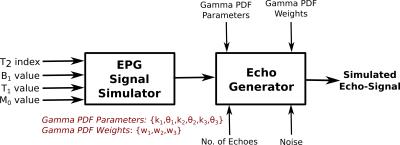
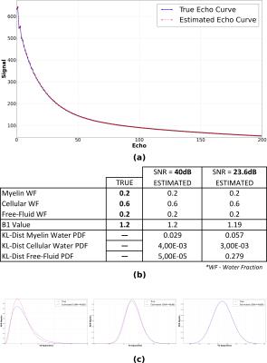
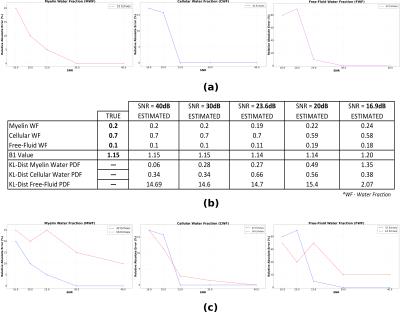
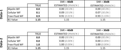
The proposed method was tested on synthetic data to assess its performance on known quantities. Generation of synthetic data was done as shown in Figure-1. For evaluating the performance, we compute the following evaluation measures: Water Fraction (WF) and B1 value comparisons, Kullback–Leibler(KL) distance between true and estimated distributions. We design a variety of experiments to cover plausible conditions that we may encounter with real data. Experiment-1: For clinical studies, due to practical acquisition time constraints, time at which the last echo is acquired ranges from$$$\,$$$100-300ms. This does not cover the entire range of T2 values corresponding to free$$$\,$$$water. Hence, to assess the correctness of free-fluid compartment’s distribution, one data set of 200-echoes (echo-spacing=10ms) was generated. Results shown in Figure-2 demonstrate that, given an ideal acquisition, all three compartments' parameters can be estimated with very high accuracy. Experiment-2 is aimed at testing the estimation technique on synthetic data with an acquisition length similar to that of clinical scenarios. We also examine effect of added noise in signal on estimation. Synthetic data is generated with 32$$$\,$$$echoes having 8.4ms echo$$$\,$$$spacing. Results are shown in Figure-3(a),(b). We also test the effect of reducing acquisition length (i.e. number of echoes) on estimation performance. Estimation results with 16 and 32 echoes are compared in Figure-3(c). Experiment-3: Regions in the brain, like ventricles are composed almost entirely of free-fluids. This poses a challenge for the estimation framework where only a single compartment is represented in a voxel. Hence for a couple of data sets (32$$$\,$$$echoes and 8.4ms echo spacing) free$$$\,$$$fluid water fraction was assigned a value$$$\,$$$≥$$$\,$$$0.9 for the voxel. Results shown in Figure-4 demonstrate good agreement of estimated and true values.Conclusion
We presented a method to get quantitative estimation of the brain tissue microstructure. We evaluated our model against synthetic data with a variety of SNRs to test robustness of the estimation framework. The synthetic data experiments considered a variety of possibilities in brain tissues. The proposed method performs accurate estimations for realistic SNR(s). The next step is to test the performance of the method on real data and gain further insights into the proposed estimation framework.Acknowledgements
No acknowledgement found.References
1. C. Laule, I. M. Vavasour, S. H. Kolind, D. K. B. Li, T. L. Traboulsee, G. R. W. Moore, and A. L. MacKay, “Magnetic resonance imaging of myelin,” Neurotherapeutics, vol. 4, no. 3, pp. 460–484, 2007.
2. A. MacKay, C. Laule, I. Vavasour, T. Bjarnason, S. Kolind, and B. Madler, “Insights into brain microstructure from the T2 distribution,” Magnetic Resonance Imaging, vol. 24, no. 4, pp. 515–525, 2006.
3. T. Prasloski, B. Madler, Q. S. Xiang, A. MacKay, and C. Jones, “Applications of stimulated echo correction to multicomponent T2 analysis,” Magnetic Resonance in Medicine, vol. 67, no. 6, pp. 1803–1814, 2012.
4. G. Golub and V. Pereyra, “Separable nonlinear least squares: the variable projection method and its applications,” Inverse Problems, vol. 19, no. 2, pp. R1–R26, 2003.
5. Gudbjartsson, Hákon, and Samuel Patz. "The Rician distribution of noisy MRI data." Magnetic resonance in medicine 34.6 (1995): 910-914.
6. Powell, Michael JD. "The BOBYQA algorithm for bound constrained optimization without derivatives." Cambridge NA Report NA2009/06, University of Cambridge, Cambridge (2009).
Figures


