4029
An Iterative Gradient Delay Correction Method for 3D UTE Imaging1UIH America, Inc., Houston, TX, United States, 2Shanghai United Imaging Healthcare Co., Ltd., Shanghai, People's Republic of China
Synopsis
Gradient imperfections such as gradient delay can cause image distortion and artifacts in UTE imaging. In this work, we report an iterative gradient delay correction method for 3D UTE imaging that allows use of arbitrary gradient waveform model, independent calibration of x, y, and z gradients, and subject-specific delay correction with an embedded prescan. The feasibility of improved image quality using this proposed method was demonstrated by volunteer data.
Introduction
Ultrashort echo time (UTE) imaging is susceptible to factors that cause k-space trajectory deviation from design, such as due to gradient delay, eddy currents, and imperfections in gradient amplifier. Various methods for gradient delay correction have been previously reported 1-3. This study proposes a different approach for gradient delay correction in 3D UTE imaging that permits the free use of gradient waveform model and independent calibration of the three physical gradient axes, which can be easily implemented as prescan and allows subject specific delay correction without the need for additional calibration.Methods
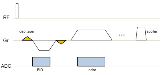
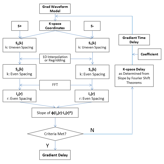
A prototype 3D multi-echo spoiled gradient-echo sequence was developed to support ramp sampling for center-out UTE acquisition. In the prescan a small dephaser gradient was added before the UTE gradient to form a partial echo for delay correction, similar to a previous publication 1. For each physical axis, the above module was repeated with positive and negative gradient polarity, resulting in two partial echo signals Sp and Sn, respectively, and then iterative data analysis was used as depicted in Figure 2. After incorporating a chosen gradient waveform model, k-space coordinates were initially determined and assigned to corresponding signals in Sp and Sn and then either 1D interpolated or regridded to positions on evenly spaced grid for Fast Fourier Transform. Next by using Fourier Shift Theorems and calculating the slope of phase difference in image space, an effective delay in k-space can be obtained. To further translate the effective k-space delay to its root cause - gradient delay in time, a coefficient is multiplied to account for the dense and uneven sampling around k-space center as a result of ramp sampling. We simply used a coefficient of 1.5 in the study though more sophisticated methods should exist. The iterations stopped when a chosen criteria was met, which was set to 20 iterations in our case and was proven to be enough. After gradient delay was acquired and k-space trajectory was determined on each physical axis separately, the trajectory of spokes off the physical axes was calculated.
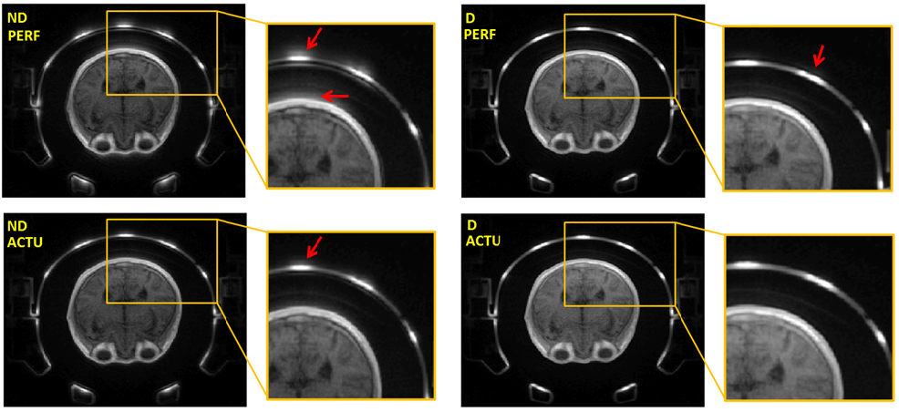
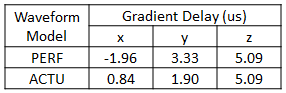
To illustrate effects of the proposed correction, UTE data were reconstructed with and without delay correction. To further demonstrate the freedom in choosing gradient waveform model, two options were sought: 1) assuming perfect trapezoid (PERF), and 2) assuming the actual waveform (ACTU) obtained with a phantom using the waveform measurement technique by Duyn, et al. 4.
Imaging was performed on a 3.0T uMR770 system (Shanghai United Imaging Healthcare, Shanghai, China). The sequence employs a 40us hard pulse for excitation. Following UTE echo acquisition two gradient echoes were formed. Other imaging parameters were: TR 4.7ms, TE1(UTE) 70us (center of the RF to the start of acquisition), TE2/TE3 2.1/3.45ms, spatial resolution 1.17*1.17*1.17mm3, RF spoiling, flip angle 10°, 155 samples were acquired during UTE with a sampling interval of 4us, 16384 spokes in total. Total imaging time was 77s. Reconstruction was done offline using regridding with Kaiser-Bessel kernel. Post density compensation was used.
Results
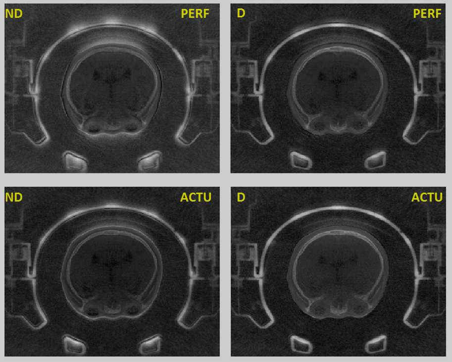
Gradient delay of x, y, and z axis calculated using the proposed method were shown in Table 1. Volunteer UTE images (Fig. 3) were reconstructed without (ND) and with gradient delay (D), and assuming PERF waveform and actual ACTU waveform, respectively. It was obvious delay corrected images have fewer artifacts and improved image quality than non-corrected images. For better visualization of cortical bone structures, log(TE1)-log(TE2) images (Fig.4) were shown. Similar conclusion can be drawn regarding the effects of delay correction and waveform choices.Discussions
An iterative gradient delay correction method in 3D UTE was proposed and its feasibility was demonstrated with improved image quality in a volunteer after correction. Because the iterations only involve 1D data and in our experience 20 iterations were already good enough, the additional time cost of this approach should be minimal. Also it was worth mentioning even incorporating actual waveform measured by Duyn technique, there were still artifacts without gradient delay correction, likely emphasizing the importance of subject-specific delay correction using a prescan.Acknowledgements
No acknowledgement found.References
[1] Herrmann KH, Krämer M, Reichenbach JR. Time Efficient 3D Radial UTE Sampling with Fully Automatic Delay Compensation on a Clinical 3T MR Scanner. PLoS One. 2016 Mar 14;11(3):e0150371.
[2] Takizawa M, Hanada H, Oka K, et al. A robust ultrashort TE (UTE) imaging method with corrected k-space trajectory by using parametric multiple function model of gradient waveform. IEEE Trans Med Imaging. 2013 Feb;32(2):306-16.
[3] Ianni JD, Grissom WA. Trajectory Auto-Corrected image reconstruction. Magn Reson Med. 2016 Sep;76(3):757-68.
[4] Duyn JH, Yang Y, Frank JA, van der Veen JW. Simple correction method for k-space trajectory deviations in MRI. J Magn Reson. 1998 May;132(1):150-3.
Figures