Introduction

Dual-echo subtraction MRI with zero echo time (DE-ZTE) provides contrast for samples with short transverse relaxation times [1]. To attain a high quality subtraction image, it is critical to correct for gradient delays and phase offsets induced by eddy currents in the gradient hardware. Relative phase correction is a data-driven approach to estimate the TE shift arising from gradient delay and phase offset arising from eddy currents [2]. However, this approach is based on linear phase fitting on the relative phase between projection pairs in image domain, which is not highly reliable. TE shifts and phase offsets can be obtained externally by means of field camera measurements [3]. However, the field probes suffer from significant signal dephasing at high resolution DE-ZTE scans, making trajectory measurements difficult. In this work, we show that the gradient delay can be accurately modeled as a linear function of gradient strength. Moreover, we show that it is possible to reconstruct high resolution DE-ZTE images to a high quality without the need for measuring trajectories at the full gradient strength.

Methods

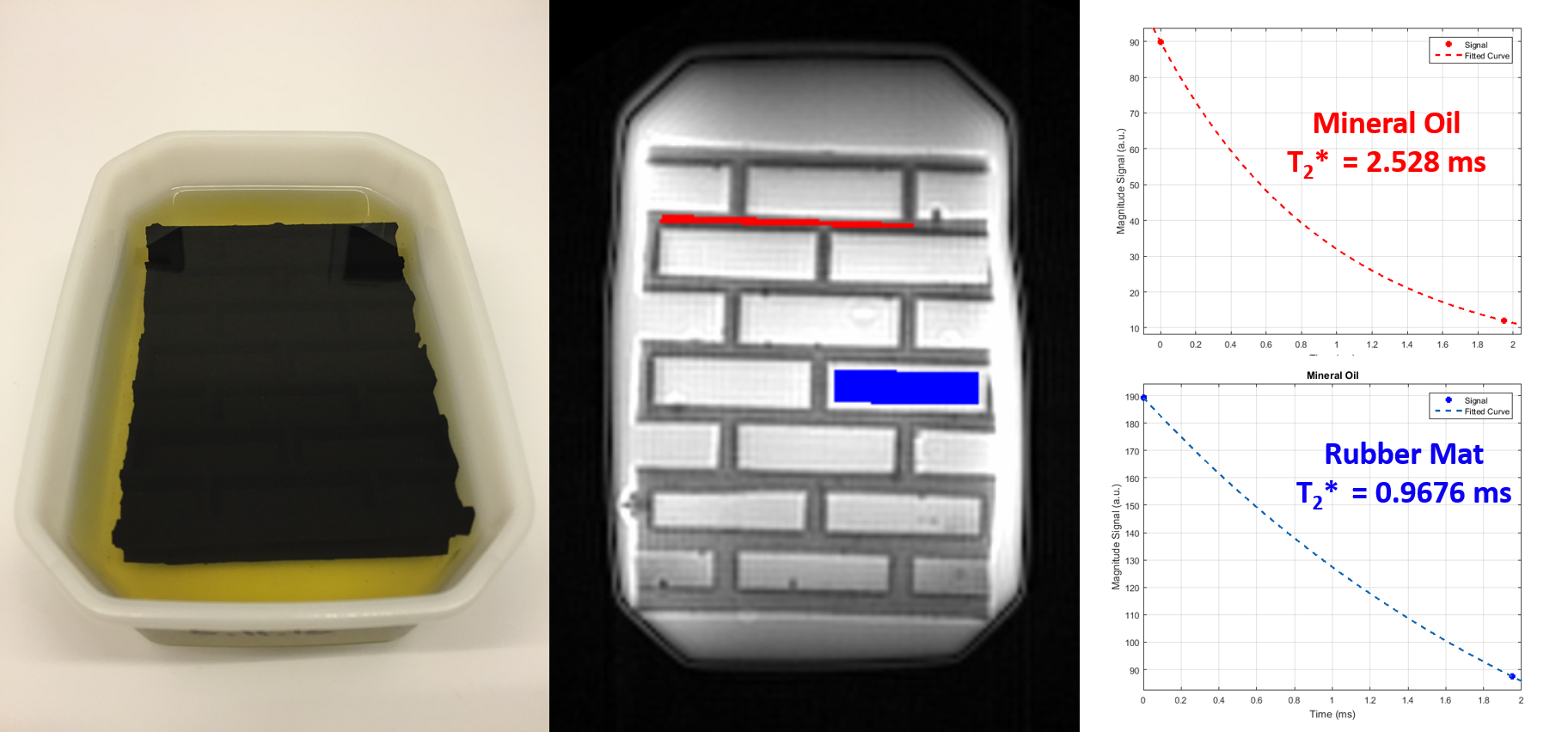
Trajectories were measured using proton field probes (T₂^* = 1.5 ms) as described in [3]. Actual TE is extracted based on the time point at which the first-order k terms cross zero for every TR in DE-ZTE scans. To compute subtraction image (SUB), weighted GRE image was subtracted from ZTE image. The weight is given by exp(-TE / T_{2_threshold}) and T_{2_threshold} of 2.2 ms was selected. The T₂^* of mineral oil was 2.528 ms and that of rubber mat was 0.9676 ms. For low resolution DE-ZTE scans, the following parameters were used: G = 24.4652, BW = 250 kHz, Voxel size = 2 mm isotropic, Matrix size = 120, nDummy = 2000, nPro = 46080, nInt = 2, dwell time = 4 us, NSA = 1, TE = 2 ms, TR = 5 ms, RF pulse duration = 2 us, Scan time = 4:01 min. For high resolution DE-ZTE scans, the following parameters were used: G = 24.4652, BW = 250 kHz, Voxel size = 1 mm isotropic, Matrix size = 240, nDummy = 2000, nPro = 184320, nInt = 2, dwell time = 4 us, NSA = 1, TE = 2 ms, TR = 5 ms, RF pulse duration = 2 us. Scan time = 15:32 min.

Results

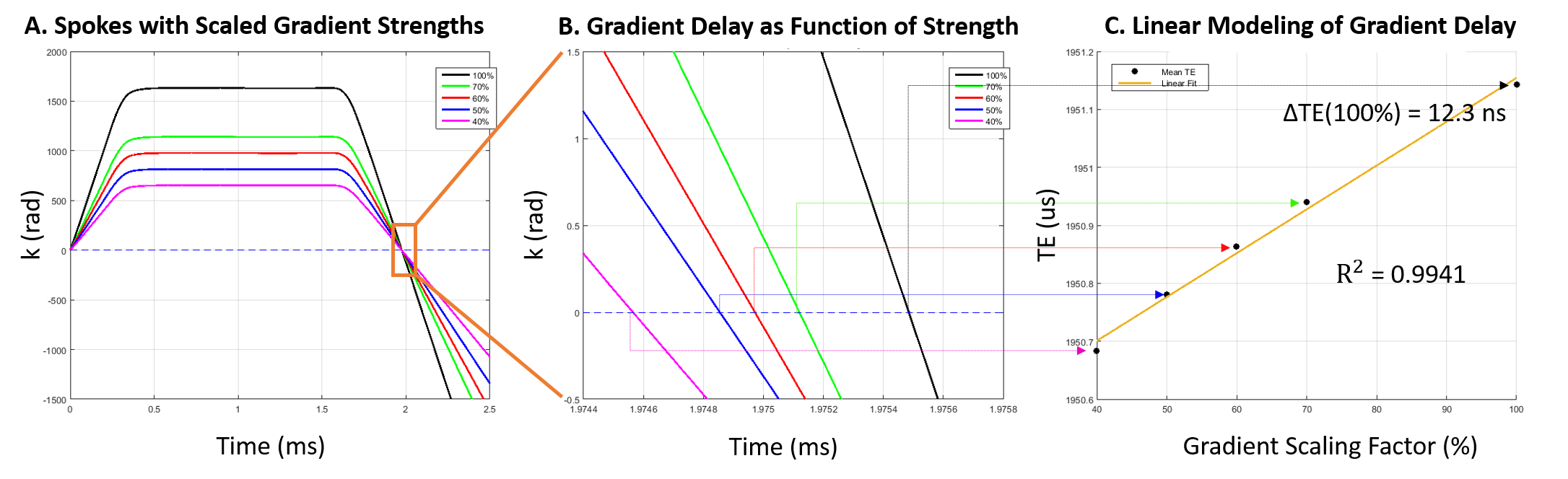
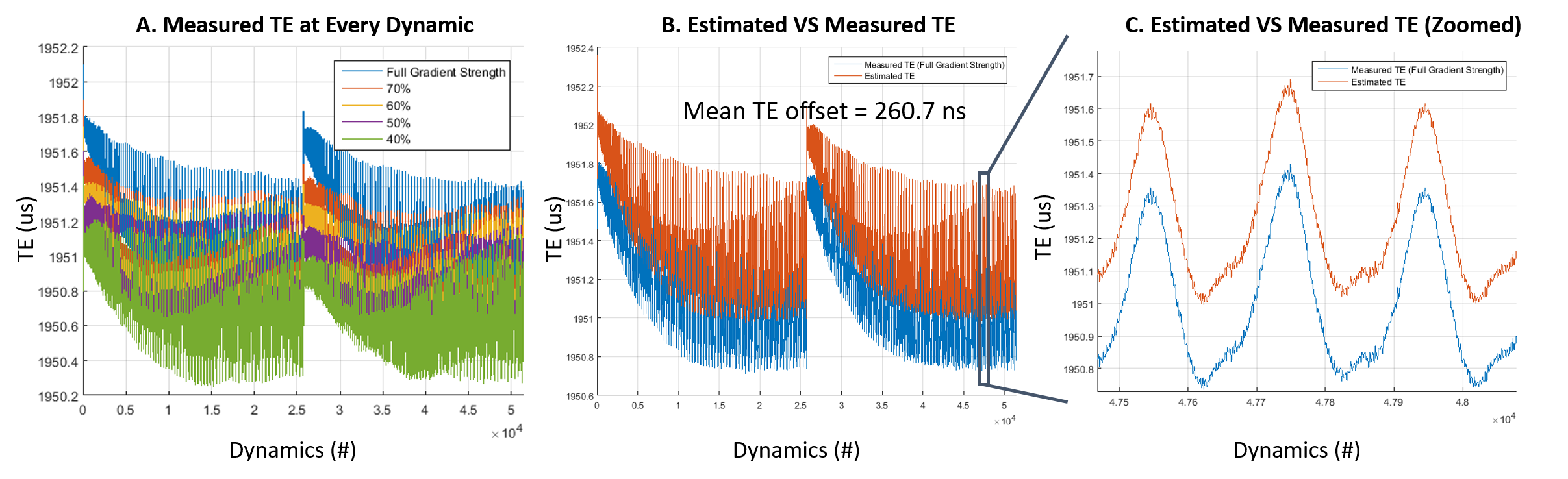
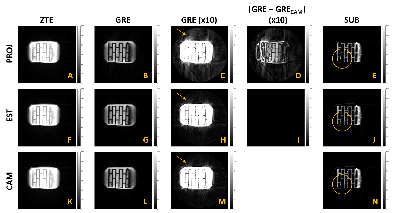
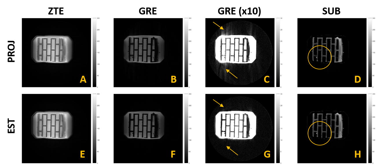
Trajectories measured at scaled gradient strengths (Fig 1A) showed that gradient delays was linearly proportional to gradient strength (Fig 1B-C). To examine this closely, a linear line was fitted to TE's acquired at multiple scaled gradients (Fig 1C). The R-squared value was 0.9941, indicating strong linear relationship and the TE offset at the full gradient strength was only 12.3 ns (Fig 1C). TE's measured at multiple scaled gradient strengths were modeled to estimate TE at the full gradient strength (Fig 2B). The mean offset was 260.7 ns, which is far shorter than the acquisition bandwidth (= 4 us), thus not expected to degrade the reconstruction performance. The estimated TE curve also shows remarkable similarity to measured TE (Fig 2C). As expected from the high accuracy of TE estimation, DE-ZTE images reconstructed based on estimated TE (EST) produced almost identical results (Fig. 4G-J) as those reconstructed based on measured TE (CAM; Fig. 4L, 4M, 4N). On the other hand, DE-ZTE images reconstructed based on projection-based TE estimation (PROJ) showed lower performance (Fig B-E) compared to EST and CAM. In high resolution DE-ZTE scans, EST performed noticeably better than PROJ (Fig. 5). In GRE images, PROJ showed artifacts in the areas indicated by yellow arrows (Fig 5C) whereas the EST-based GRE image showed no artifact in the same area (Fig. 5G).

Conclusion

We demonstrated that gradient delay can be accurately modeled as a linear function of gradient strength and that it can be successfully applied to DE-ZTE reconstruction at high resolution. This may potentially allow estimating gradient delays at higher resolution as well as finding other applications where correcting for gradient delays play an important role.

Acknowledgements

No acknowledgement found.