Synopsis

Gridding is a relevant algorithm for both image reconstruction and pulse design. With Gridding, it is crucial to appropriately compensate for varying density of the sampling trajectory. In this paper, we present a technique to determine the weights by solving a least squares optimization problem.

Purpose

Theory

The Gridding algorithm is encapsulated in the following expression [4]:

\begin{equation} \hat{f}(n) = \frac{1}{c(n)}\text{DFT}^{-1}\left\{ \mathcal{T}\left[ (F\,S_w \circledast C) \text{III}_{\Delta k/\alpha} \right] \right\}[n], \end{equation}

where $$$F$$$ is the Fourier transform of the image $$$f$$$, $$$\hat{f}$$$ is a vector of estimates of $$$f$$$, $$$\text{III}$$$ is the comb function, $$$S_w(k)=\sum w_i\, \delta(k-k_i)$$$ (a distribution of weighted impulse functions), $$$\circledast$$$ represents a circular convolution, $$$C$$$ is the Gridding convolution kernel, $$$c$$$ is the deapodization function, $$$\alpha$$$ is the oversampling factor, and $$$\mathcal{T}$$$ is an isomorphism that maps the non-zero values of $$$F\,S_w$$$ to a vector in $$$\mathbb{C}^M$$$. In [5], Pipe et al. suggest determining the density compensation function with the following Fixed Point (FP) iteration:

\begin{equation*} diag(w_{i+1}) = diag(w_i) \, diag^{-1}\left( \mathcal{C} w_i \right)\end{equation*}

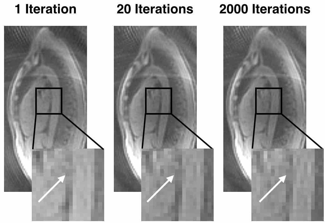
where $$$\mathcal{C}$$$ is the linear transformation that convolves the distribution of weighted impulse functions $$$S_w(k)=\sum\delta(k-k_i)$$$ with the Gridding kernel and evaluates the result on sample points. Intuitively, if $$$S_w^{(i)}\ast C\approx\boldsymbol{1}$$$ at all points in the support of $$$S_w$$$ then $$$S_w^{(i+1)}\approx S_w^{(i)}$$$. FP attempts to set the weights so that value before and after convolution with the Gridding kernel at all $$$k\in\boldsymbol{k}$$$ remains constant. However, this algorithm is not guaranteed to converge; the authors suggest running for 15 iterations, but figure 1 shows an example where the solutions after 1, 15, and 2000 iterations differ.

We propose to determine the weights by solving the following Least Squares problem:

\begin{equation*} \text{minimize} \hspace{8pt} \| \mathcal{C} \, w - \boldsymbol{1} \|_2. \label{eq:LSDC}\end{equation*}

Solving this problem also seeks to make $$$\mathcal{C}\,w\approx\boldsymbol{1}$$$. Importantly, though, this problem can be solved with efficient numerical algorithms (such as LSQR [7]). We call this algorithm Least Squares Density Compensation (LSDC); when compared to FP, it eliminates the requirement that a user specify the number of iterations (though a stopping criteria is required), and it is guaranteed to converge to an optimal solution (in a Least Squares sense).

Results

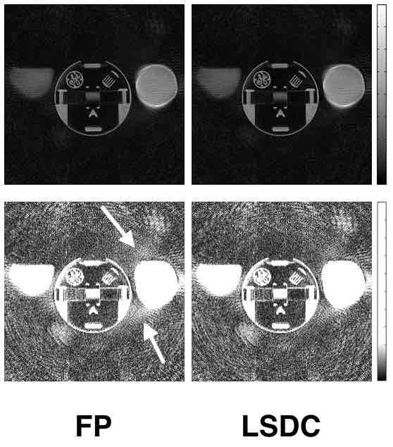
Figure 2 presents Gridding results of data collected with a phantom using a 2D radial trajectory with 418 radial lines, a field of view of 29 cm, and a resolution of 1.1 mm collected with a 1.5T scanner. There is an improvement in quality when LSDC is used instead of FP; the arrows point to regions where LSDC is able to reduce the amount of noise present in the imagery.

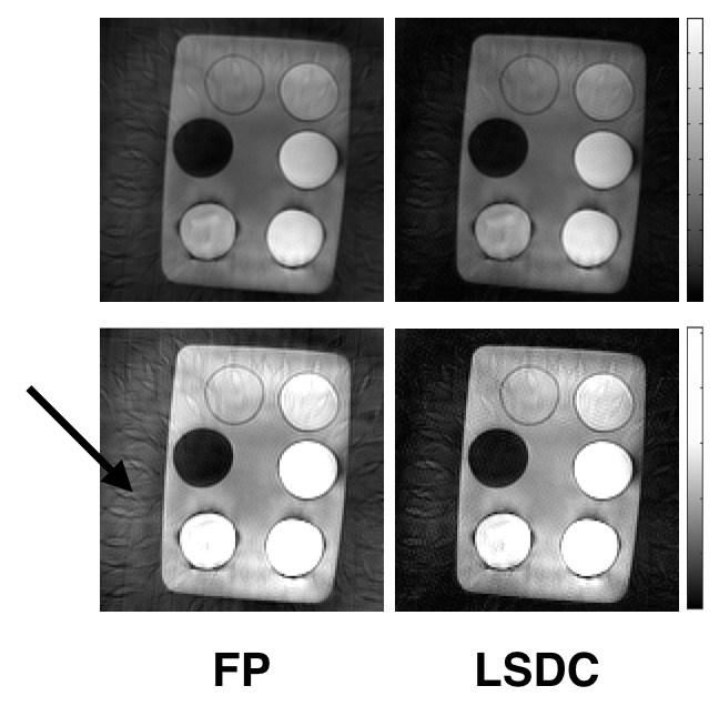
Figure 3 presents Gridding results of data collected with a phantom comprised of six bottles of varying substances using a propeller trajectory with 159 points per readout, 20 lines per angle, and 22 angles (each separated by the golden angle) collected with a 1.5T scanner. Again, there is an improvement in quality when LSDC is used. In addition to the area indicated by the arrow, there is a bright halo that is significantly reduced by LSDC.

Conclusion

Acknowledgements

ND is supported by the National Institute of Health's Grant Number T32EB009653 “Predoctoral Training in Biomedical Imaging at Stanford University”, the National Institute of Health's Grant Number NIH T32 HL007846, The Rose Hills Foundation Graduate Engineering Fellowship, the Electrical Engineering Department New Projects Graduate Fellowship, and The Oswald G. Villard Jr. Engineering Fellowship.

References

[1] John I. Jackson, Craig H. Meyer, and Dwight G. Nishimura. Selection of a Convolution Function for Fourier Inversion Using Gridding. IEEE Transactions on Medical Imaging, 10(3), September 1991.

[2] Christopher J Hardy, Harvey E Cline, and Paul A Bottomley. Correcting for Nonuniform K-space Sampling in Two-dimensional NMR Selective Excitation. Journal of Magnetic Resonance (1969), 87(3):639–645, 1990.

[3] JD O’sullivan. A Fast Sinc Function Gridding Algorithm for Fourier Inversion in Computer Tomography. Medical Imaging, IEEE Transactions on, 4(4):200–207, 1985.

[4] Philip J Beatty, Dwight G Nishimura, and John M Pauly. Rapid Gridding Reconstruction with a Minimal Oversampling Ratio. Medical Imaging, IEEE Transactions on, 24(6):799–808, 2005.

[5] James G Pipe and Padmanabhan Menon. Sampling Density Compensation in MRI: Rationale and an Iterative Numerical Solution. Magnetic Resonance in Medicine, 41(1):179–186, 1999.

[6] Holden H Wu, Bob S Hu, Dwight G Nishimura, and Michael V McConnell. Multi-phase Coronary Magnetic Resonance Angiography Using a 3D Cones Trajectory. Journal of Cardiovascular Magnetic Resonance,13(1):1, 2011.

[7] Christopher C Paige and Michael A Saunders. LSQR: An Algorithm for Sparse Linear Equations and Sparse Least Squares. ACM Transactions on Mathematical Software, 8(1):43–71, 1982.