4008
Implementation and Optimization of an Automatic k-Space Trajectory Correction for Ultrashort Echo Time Imaging1MR-Imaging and Spectroscopy, University of Bremen, Bremen, Germany, 2Fraunhofer MEVIS, Bremen, Germany
Synopsis
Ultrashort echo time (UTE) sequences are usually applied for imaging of very short T2* tissues, for the evaluation of water content in the cortical bone and for X-nuclei imaging. The aim of this study was the implementation of an automatic calibration measurement to determine the actual k-space trajectory considering noisy data samples in UTE imaging. In contrast to most other studies, not only gradient delays were taken into account, but also gradient waveform distortions. It could be demonstrated that there exist an optimal number of samples used for correction (depending on signal-to-noise ratio) that should be determined by calibration scans.
Introduction
Ultrashort echo time (UTE) sequences are usually applied for imaging of very short T2* tissues1,2, for the evaluation of water content in the cortical bone3,4 and for X-nuclei imaging5. Non-Cartesian image reconstruction is challenging because of the gridding procedure and k-space trajectory correction. Minimal k-space trajectory deviations due to gradient imperfections lead to a bunch of image artifacts such as blurring and signal displacements. Most studies correct for gradient delays, but eddy currents also result in distorted gradient waveforms, which have to be corrected for optimal image quality. The aim of this study was the implementation of an automatic calibration measurement to determine the actual k-space trajectory considering noisy data samples.Methods
All measurements were performed on a 3 T whole-body MR scanner (MAGNETOM Skyra, Siemens Healthcare, Erlangen, Germany) with a 16-channels head coil, of which eight channels were used for data acquisition.
A 3D radial UTE sequence was applied to obtain images of a spherical water phantom with 1.25 wt‰ NiSO4 at an isotropic resolution of 1 mm. Acquisition parameters were as follows: repetition time = 5 ms, echo time = 60 μs, flip angle = 5°, 30,000 projections, 160 samples per projection, readout time = 700 μs. A maximum gradient strength of 18.2 mT/m was needed at a maximum slew rate of 170 T/m/s. A ‘negative ADC delay’ of 10 μs was employed to discard the first two defective sample points. 300 prescans were applied to reach the steady-state before data acquisition. Correction of the k-space trajectory was performed according to Duyn et al.6 using four different slice distances (±2, ±4 cm) with 3 mm slice thickness and five averages along each axis. The data of the eight channels were compressed to two virtual channels7. Data were gridded for a field-of-view (FOV) of 200 mm with a Kaiser-Bessel kernel8, oversampling ratio9 of 1.375 and sample density precompensation followed by Hamming-filtering. All reconstruction steps were implemented on the scanner’s hardware. Data gridding starts directly so that images are available 10 seconds (depending on matrix size and number of channels) after the measurements with the above-mentioned parameters have finished.
Image reconstruction was performed with the above-mentioned k-space trajectory correction, whereas a different number of the first data samples were considered for correction. For the remaining samples, the correction factor of the last considered sample point was applied. Since a homogeneous water phantom was measured, signal should be composed of a constant water signal and noise, if partial-volume effects and coil sensitivity can be neglected. Thus, the entropy $$$E$$$ was used as a measure of signal homogeneity$$E=-\sum_{i=1}^{256}{p_i\textrm{log}_2(p_i)},$$where signal strengths are subdivided into 256 bins and $$$p_i$$$ counts the pixel of the $$$i$$$-th interval.
One measurement was performed in the human brain with the above-mentioned parameters except a repetition time of 6 ms, a FOV of 220 mm, acquisition of two echoes (TE1 = 60 μs, TE2 = 1.8 ms) and the application of a fat saturation pulse before each 10th RF excitation. A difference image ∆I of both contrasts was calculated as follows: ∆I = 0.75 · I(TE1) - I(TE2) .
Results & Discussion
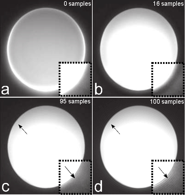
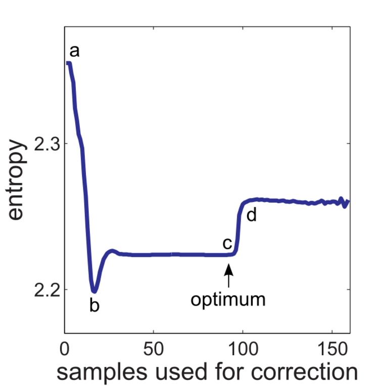
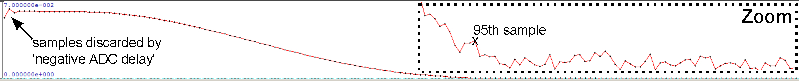
Figure 1 shows the phantom measurement without (Fig. 1a) and with correction considering a different number of data samples (Figs. 1b-d). A strong image degradation is visible without correction and optimal image quality can be obtained for 95 samples, which can also be demonstrated by the entropy in Figure 2 (point c). The entropy minimum at point b is not optimal (cf. Figs. 1b,c) and can be explained by the coil profile. Since signal is pushed outwards without correction, the signal inside the phantom appears more homogeneous resulting in a lower entropy. The increased entropy and worse image quality from point d can be explained by non-sufficient raw data signal at the outer k-space (cf. Fig. 3). Six calibration scans without RF excitation were performed to determine the noise level and to automatically select the optimal number of samples used for correction. Figure 4 shows two echoes and their weighted difference image of a human brain measurement, whereas 0, 80, and 90 samples are considered for correction. Best performance could be obtained with the automatically detected optimal number of 80 sample points.Conclusion
A fully automatic k-space trajectory correction on the scanner’s hardware for UTE imaging is presented. In contrast to most other studies, not only gradient delays were taken into account, but also gradient waveform distortions. Furthermore, it could be demonstrated that there exist an optimal number of samples used for correction (depending on signal-to-noise ratio) that should be determined by calibration scans.Acknowledgements
No acknowledgement found.References
1. Robson MD, Gatehouse PD, Bydder M, Bydder GM. Magnetic resonance: An introduction to ultrashort TE (UTE) imaging. J Comput Assist Tomogr 2003;27:825-846.
2. Chang EY, Du J, Chung CB. UTE imaging in the musculoskeletal system. J Magn Reson Imaging 2015;41:870-883.
3. Du J, Bydder GM. Qualitative and quantitative ultrashort-TE MRI of cortical bone. NMR Biomed 2013;26:489-506.
4. Bae WC, Chen PC, Chung CB, Masuda K, D’Lima D, Du J. Quantitative ultrashort echo time (UTE) MRI of human cortical bone: Correlation with porosity and biomechanical properties. J Bone Miner Res 2012;27:848-857.
5. Konstandin S, Nagel AM. Measurement techniques for magnetic resonance imaging of fast relaxing nuclei. Magn Reson Mater Phys 2014;27:5-19.
6. Duyn JH, Yang Y, Frank JA, van der Veen JW. Simple correction method for k-space trajectory deviations in MRI. J Magn Reson 1998;132:150-153.
7. Huang F, Vijayakumar S, Li Y, Hertel S, Duensing GR. A software channel compression technique for faster reconstruction with many channels. Magn Reson Imaging 2008;26:133-141.
8. Jackson JI, Meyer CH, Nishimura DG, Macovski A. Selection of a convolution function for Fourier inversion using gridding. IEEE Trans Med Imag 1991;10:473-478.
9. Beatty PJ, Nishimura DG, Pauly JM. Rapid gridding reconstruction with a minimal oversampling ratio. IEEE Trans Med Imag 2005;24:799-808.
Figures