4004
Comparison of Sequential and Joint Methods for Spiral Water-fat Separation and Deblurring1Imaging research, Barrow Neurological Institute, Phoenix, AZ, United States
Synopsis
Most previous approaches to spiral water-fat imaging perform the water-fat separation and deblurring sequentially based on the assumption that the phase accumulation and blurring are separable. A joint water-fat separation and deblurring method has been recently proposed using more accurate signal models. In this study, the sequential and joint methods are quantitatively compared. Simulation and experiments have demonstrated that the results of the joint method are significantly better in regions where the field inhomogeneity changes rapidly in space. The loss of signal-to-noise-ratio is minor for both approaches at optimal TEs when the noise in the field map Δf0 is negligible.
Introduction
One major challenge of spiral water-fat imaging is that the static field inhomogeneity (Δf0) and the chemical shift of fat cause phase accumulation as well as blurring in images. Most previous approaches1,2 perform water–fat separation and deblurring sequentially. That is, the water and fat are first separated as if they were not blurred, and then the water and fat images are deblurred separately. The sequential approach might work well if the field map Δf0 varies slowly in space. However, in regions where Δf0 changes rapidly, water and fat signals may blur into various locations that have very different Δf0 compared to the original location. As a result, the reconstructed water and fat can be inaccurate even with a perfectly known Δf0 map. In order to address this issue, a joint water-fat separation and deblurring method has been proposed.3, 4 The purpose of this work is to quantitatively compare the joint and the sequential approaches by simulation and experiments.Methods
Spiral k-space data at 3 Tesla were simulated using discrete Fourier transform, from which blurred images were reconstructed. The field map Δf0 has a localized rapidly varying region as shown in Fig.1 (a). In both sequential and joint methods, deblurred images are resolved using a conjugate gradient method4, in which the procedures of blurring and deblurring are implemented by spatially varying convolution5. The root mean square error (RMSE) between the deblurred and the reference images was normalized by the mean magnitude of the reference images to yield the normalized RMSE (NRMSE).
Independent noise was simulated in k-space to yield blurred source images with SNR around 20. In the first method (method 1), noise was added to the spiral k-space data 100 times to estimate the noise standard deviation (STD) at each pixel. In the second method (method 2), a separate set of noise k-space data was generated. The noise data were post-processed exactly the same as the image data.6 STD of the noise was estimated in a 10×10 window for each pixel. SNR was evaluated in three ROIs, each of which includes 50×50 pixels. Then the relative SNR of water was obtained by the ratio of the SNR of the deblurred water and the SNR of the mean of the source magnitude images at multiple TEs. Noise was also added to Δf0 to investigate its effect on the deblurring with noiseless source images.
T1-weighted gradient-echo data were collected for three volunteers using distributed spirals7 on a 3T Philips Ingenia scanner with a 15-channel head coil. In all scans, data were acquired at two TEs with ΔTE=1.15 ms. Δf0 maps were obtained from a separate low-resolution scan.8 Pure noise data sets were also acquired6 for SNR evaluation using method 2.
Results and Discussion
Fig. 1 shows that the joint method visibly outperforms the sequential method where Δf0 varies rapidly (inside the yellow box in Fig.1). NRMSEs of the joint method are significantly lower in this area (Fig. 2). The NRMSE values of the joint method are also lower in regions with slow varying Δf0, although the difference is much more subtle.
When an error threshold is utilized as the local convergence criterion, the overall SNR increases (Fig 3 (b)) at a possible trade-off of slightly decreased accuracy for fat (Fig2 (b)). SNR values estimated by method 2 are close to that of method 1 (Fig. 3 (a)(b)). The maximum difference of the two is less than 4% when the error threshold is set to 5%, according to four simulated data sets with readout time ranging from 6.7 ms to 19.5 ms. For both deblurring methods, the maximum SNR can be obtained with ΔΤΕ around 1.2 ms and 0.7 ms for two-point and three-point acquisitions, respectively (Fig.3 (c)(d)). SNR decreases dramaticlly with the increment of noise in Δf0. Fig.3 (e) suggests that the degradation of SNR cannot be ignored when STD of Δf0 is more than 2 Hz.
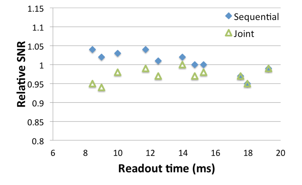
Experimental results demonstrate that the joint method consistently performs better in regions with rapidly changing Δf0, as indicated in one example shown in the circled area in Fig. 4. . The relative SNRs estimated from various volunteer scans slightly fluctuate between 0.94-1.03 (Fig. 5), which is consistent with the simulation.
Conclusions
The joint approach improves water-fat separation and deblurring significantly
where Δf0 changes rapidly. The SNR cost for both approaches is minor when
optimal TEs are used.
Acknowledgements
This work was funded by Philips Healthcare.References
1. Börnert P, van Zyl S, Eggers H, et al. Fast single breath-hold 3D abdominal spiral imaging with water / fat separation and off-resonance correction. In Proceedings of the 17th anunual meeting of ISMRM, Hawaii, United Sates, 2009. p. 2148.
2. Börnert P, Koken P, and Eggers H. Spiral water-fat imaging with integrated off-resonance correction on a clinical scanner. J Magn Reson Imaging, 2010; 32(5): 1262–1267.
3. Zwart NR, Wang D, and Pipe JP. Spiral CG deblurring and fat-water separation using a multi-peak fat model. In Proceedings of the 22th anunual meeting of ISMRM, Milan Italy, 2014. p. 1660.
4. Wang D, Zwart NR, Li Z, et al. Analytical three-point Dixon method: With applications for spiral water-fat imaging. Magn Reson Med, 2016; 75(2):627–638.
5. Ahunbay E and Pipe JP. Rapid method for deblurring spiral MR images. Magn Reson Med, 2000; 44(3): 491–494.
6. Yu J, Agarwal H, Stuber M, et al. Practical Signal-to-Noise Ratio Quantification for Sensitivity Encoding: Application to Coronary MRA. J Magn Reson Imaging, 2011; 33(6):1330–1340.
7. Turley DC and Pipe JP. Distributed spirals: A new class of three-dimensional k-space trajectories. Magn Reson Med, 2013. 70(2): 413–419.
8. Berglund J, Johansson L, Ahlström H, et al. Three-point dixon method enables whole-body water and fat imaging of obese subjects. Magn Reson Med, 2010; 63(6):1659–1668.
Figures
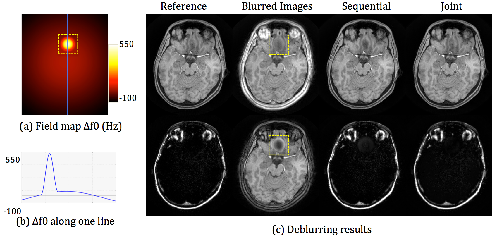
Figure 1 Simulation of water-fat separation and deblurring. One vertical line of the field map Δf0 (a) is plotted in (b). The deblurring results of the sequential and joint methods are compared in (c). The yellow boxes indicate the region where Δf0 changes rapidly. Inside this region, the sequential method yields visible inaccuracy, which is mitigated by the joint method. FOV = 240 × 240 mm2, resolution = 1 × 1 mm2. Readout time = 9.84 ms. TE = {0, 1.15} ms.
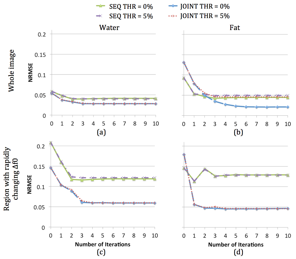
Figure 2 NRMSEs of the sequential and the joint methods are compared for the whole image (a)(b) and the region shown in Fig. 1 by a yellow box (c)(d). NRMSEs are shown in (a)(c) for water and (b)(d) for fat. Error threshold is set to 0% and 5%, respectively. SEQ: sequential approach. JOINT: joint approach. THR: threshold.
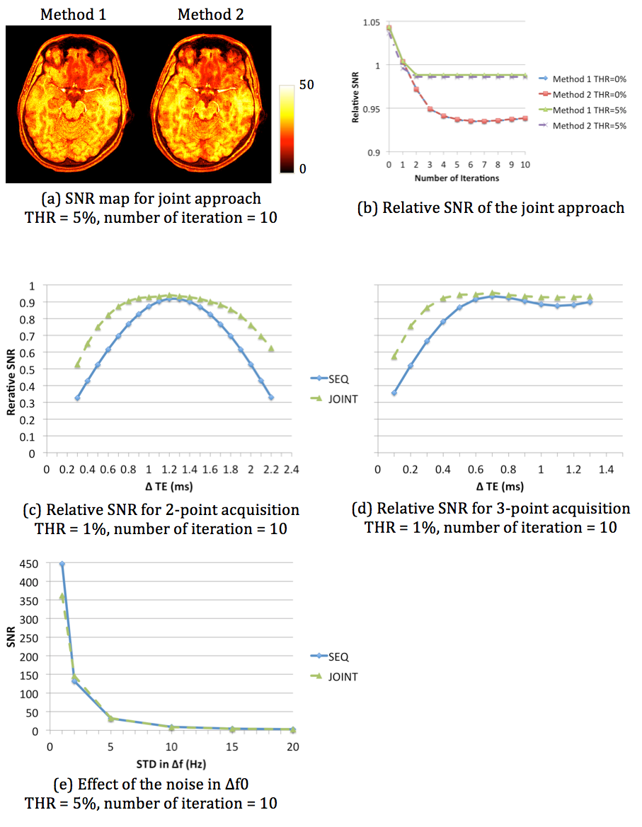
Figure 3 Results of noise simulation. Two methods yield similar noise estimations as shown in SNR maps (a) and the relative SNR plot (b). The dependence of the relative SNR on ΔTE is estimated using method 2, for two-point imaging (c) and three-point imaging (d). ΔTE1= ΔTE2 = ΔTE in three-point imaging. The SNR due to the noise in Δf0 is estimated by method 1 (e). TE1 = 0 ms and TE2 = 1.15 ms in (a) (b) and (e). SEQ: sequential approach. JOINT: joint approach. THR: threshold.
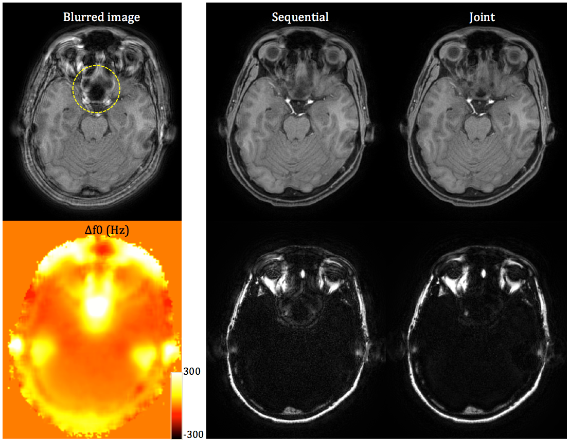
Figure 4 Comparison of the sequential and the joint approaches with experimental data. Readout time is 10.00 ms. TE = {1.13, 2.28} ms. Error threshold is 5% and maximum number of iteration is 10. Note that the joint method yields better water-fat separation and deblurring in the area in the yellow circle. FOV = 230 × 230 × 130 mm3, resolution = 1 × 1 × 2 mm3.