4002

Rapid Non-Cartesian Regularized SENSE Reconstruction using a Point Spread Function Model

Corey A Baron¹, Nicholas Dwork¹, John M Pauly¹, and Dwight G Nishimura¹

¹Stanford University, Stanford, CA, United States

Synopsis

Iterative reconstructions of undersampled non-Cartesian data are computationally expensive because non-Cartesian Fourier transforms are much less efficient than Cartesian Fast Fourier Transforms. Here, we introduce an algorithm that does not require non-uniform Fourier transforms during optimization iterations, resulting in large reductions in computation times with no impairment of image quality.

Purpose

To introduce a computationally efficient algorithm for non-Cartesian regularized SENSE that does not require non-uniform Fourier transforms during optimization iterations.

Theory

Regularized SENSE reconstructions of non-Cartesian data are typically performed by solving the following regularized weighted least-squares problem:$$(1)\quad\underset{x}{\arg\min}\left\|D(SRx-k_s)\right\|_2^2+\Phi(x)$$where $$$x$$$ is the object, the matrix $$$R$$$ represents multiplication by receiver sensitivity profiles, $$$S$$$ represents non-Cartesian k-space sampling (i.e., non-uniform Fourier transform), $$$k_s$$$ is the measured data, $$$D$$$ contains density compensation weights, and $$$\Phi$$$ is the regularization function. $$$S$$$ and its Hermitian transpose, $$$S^H$$$, must be computed every optimization iteration, and they are commonly estimated using inverse and forward gridding, respectively. Gridding and inverse gridding are computationally expensive, which makes non-Cartesian regularized SENSE reconstructions time consuming.

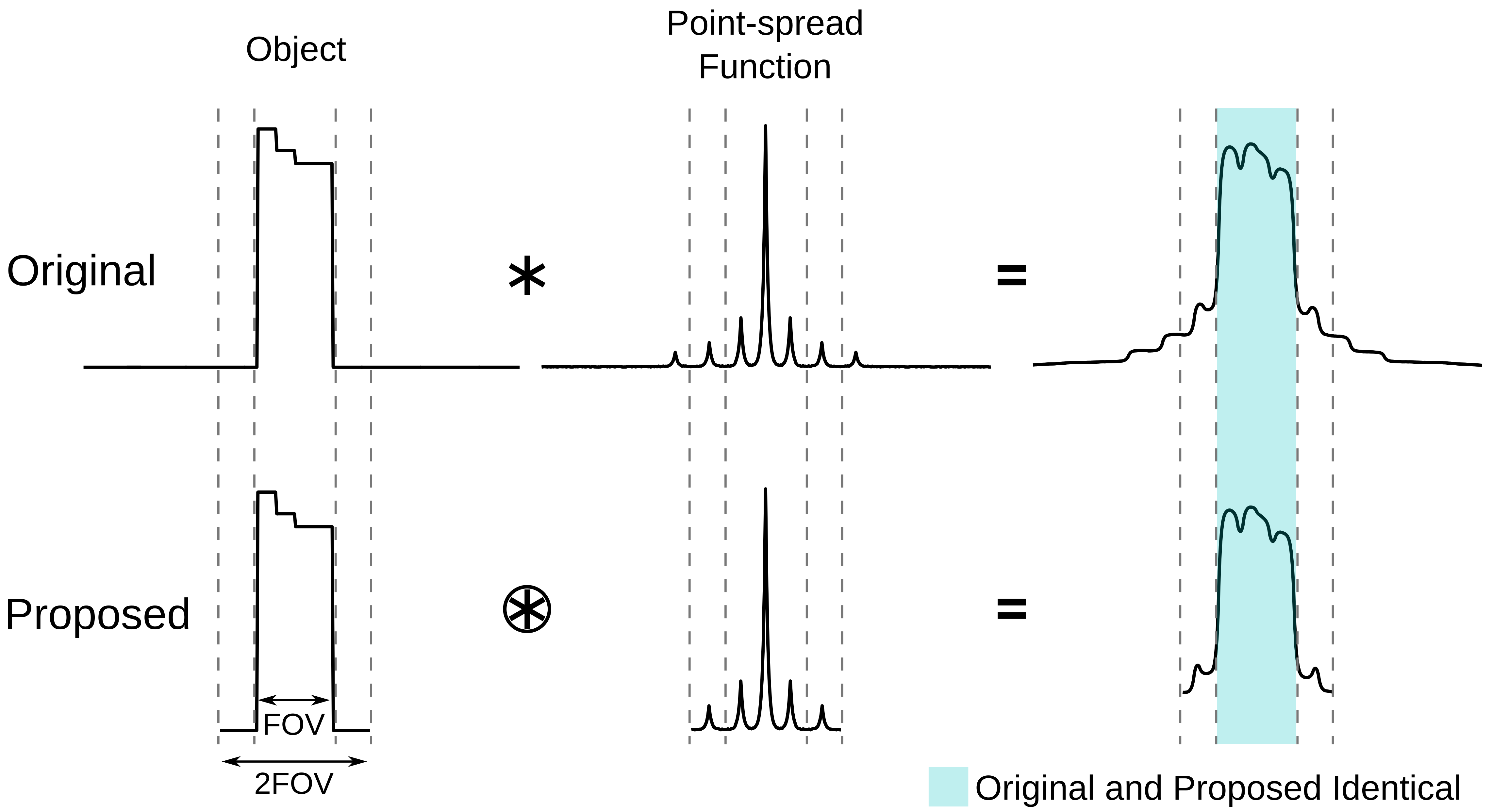
Here, we reinterpret the problem by considering the point-spread function, $$$P$$$, of the non-Cartesian sampling operation. The k-space sampling operation $$$S$$$ is equivalent to convolving $$$x$$$ with $$$P$$$ over all space. Here, we recognize that it is only necessary to estimate the result of the convolution within the FOV (i.e., where signal resides), which can be performed without leaving Cartesian sampling coordinates as long as $$$P$$$ is known to twice the FOV (Fig. 1). $$$P$$$ and its Fourier transform, $$$M$$$, can be estimated by gridding a vector of ones to 2FOV (i.e., $$$M=diag(FP)=diag(FS_{2FOV}^HD1)$$$). Then, the convolution can be computed as $$$Z^HF^{-1}MFZRx$$$, where $$$F$$$ is the FFT, $$$Z$$$ is zero-padding to 2FOV, and $$$Z^H$$$ is cropping back to the FOV. Assuming an LTI system, the result of this convolution is equal to $$$S^HDk_s$$$, which defines the problem for this method:

$$(2)\quad\underset{x}{\arg\min}\left\|Z^HF^{-1}MFZRx-S^HDk_s\right\|_2^2+\Phi(x)$$

Compared to Eq. 1, iterative inverse gridding and gridding are replaced by Cartesian Fourier transforms with 2x zero-padding and multiplication by a diagonal matrix $$$M$$$. Accordingly, gridding is performed only once to determine $$$S^HDk_s$$$ and inverse gridding is never performed. Also, $$$M$$$ is by definition real-valued and the normal equations for the least-squares solution are $$$R^HZ^HF^{-1}MFZR=R^HS^HDk_s$$$. Since Cartesian FFT’s are rapid and efficiently multithreaded, this method has the potential to improve computation times compared to Eq. 1. Notably, $$$M$$$ can be precomputed since it depends only on the k-space trajectory.

Methods

Fully sampled data was acquired using a spoiled gradient echo 3D cones trajectory [1] in a volunteer on a 1.5 T GE Signa Excite with TR = 5.5 ms, TE = 0.6 ms, flip 30°, BW = 250 kHz, FOV = 28 x 28 x 14 cm³, 1.2 mm isotropic resolution, 9137 readouts, readout duration = 2.8 ms, and 8 receiver channels. Receiver sensitivity profiles were estimated using ESPIRiT [2]. The data was retrospectively resampled to undersampled non-Cartesian trajectories using inverse gridding. Reconstructions were performed using the conjugate gradient method with Tikhonov regularization for both Eq. 1 and Eq. 2. The trajectories investigated were 3D cones with 2.15x undersampling and phyllotaxis 3D radial with 2x undersampling (same resolution and FOV as the fully sampled image). Multithreaded gridding was implemented using an oversampling ratio of 1.5 and a kernel size of 4 [3].

Results and Discussion

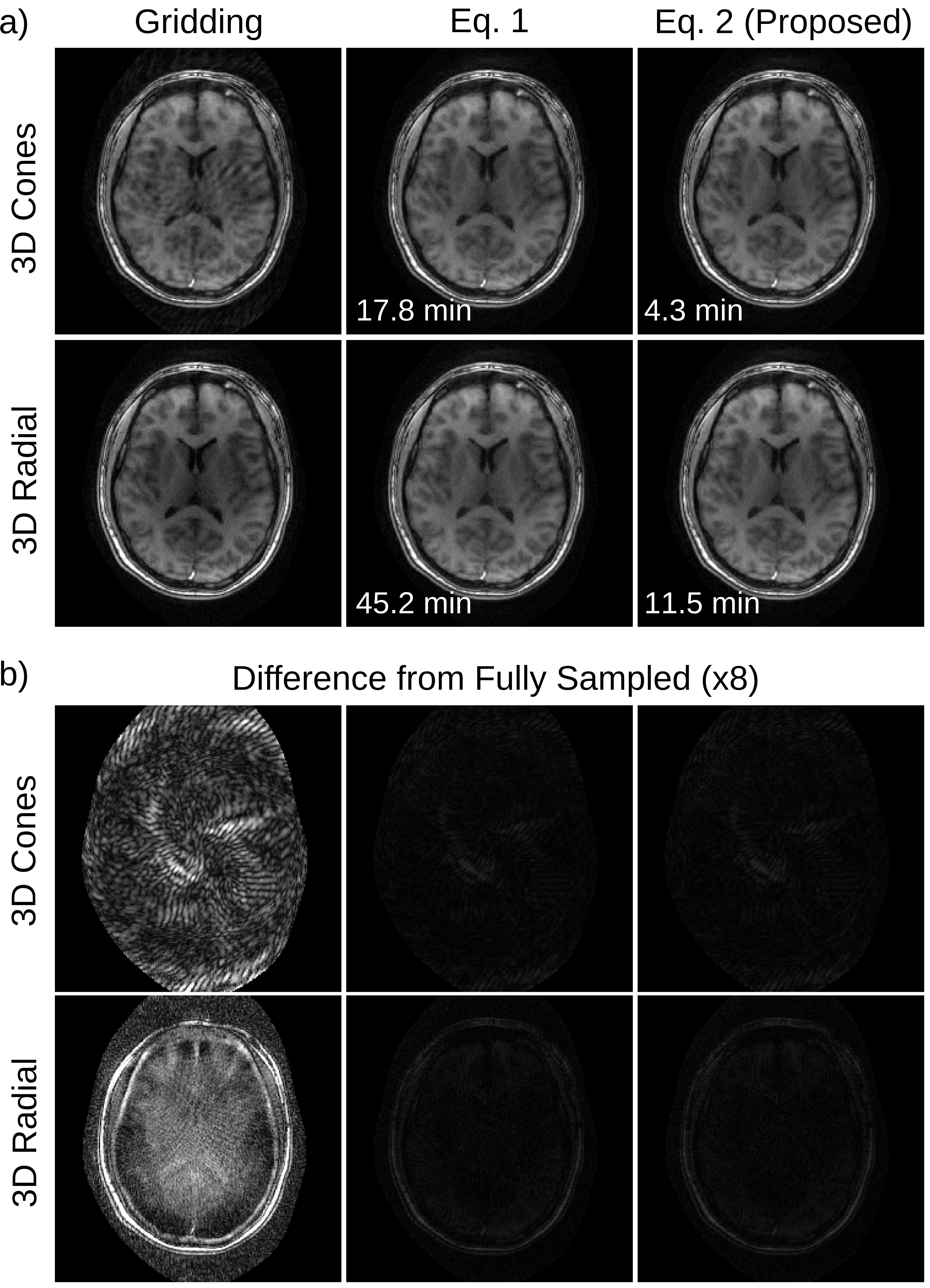
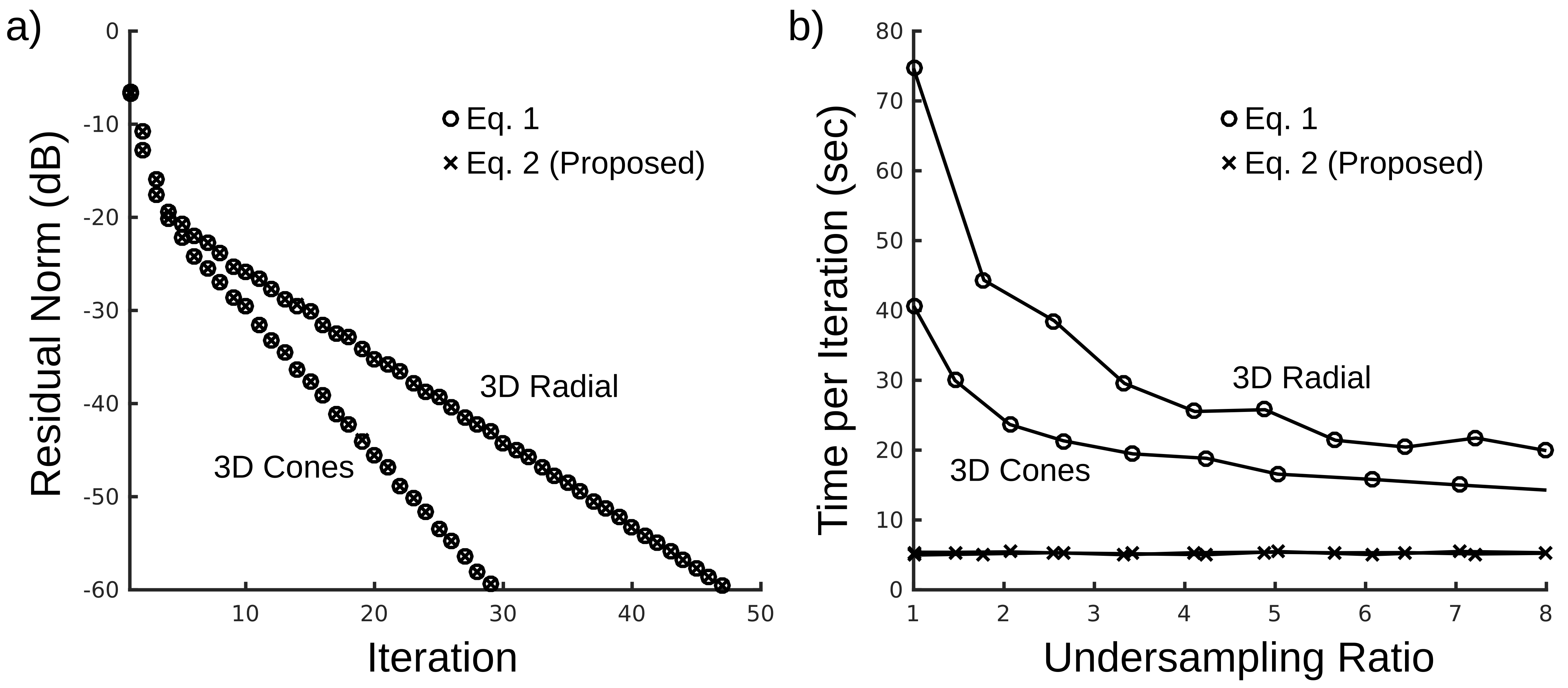
Basic gridding and regularized SENSE reconstructions using both Eq. 1 and 2 are shown in Fig. 2. Both methods give nearly identical results to each other; however, the reconstruction is approximately 4x faster for Eq. 2. Both methods also have nearly identical convergence (Fig. 3a), which suggests that Eq. 1 and 2 are equivalent to within errors of gridding and inverse gridding. The time required for one conjugate gradient iteration depends on the rate of undersampling for Eq. 1, but not for Eq. 2 (Fig. 3b); however, Eq. 2 is faster than Eq. 1 for all practical undersampling rates.

Least-square NUFFT could be used in Eq. 1 instead of gridding and inverse gridding. While NUFFT can have better speed/error ratios than Kaiser-Bessel gridding, computation times are still lengthy compared to Cartesian FFT’s. Furthermore, computation times for Eq. 1 scale dramatically with gridding/NUFFT accuracy. In contrast, computation times using Eq. 2 scale very slowly with gridding/NUFFT accuracy because gridding is only performed once (not including point-spread-function computation, which can be pre-computed).

Acknowledgements

We acknowledge the following funding sources: NIH R01 HL127039, GE Healthcare.

References

1. Wu HH, Gurney PT, Hu BS, Nishimura DG, and McConnell MV. Free-breathing multiphase whole-heart coronary MR angiography using image-based navigators and three-dimensional cones imaging. MRM 2013;69(4):1083-1093

2. Uecker M, Lai P, Murphy MJ, Virtue P, Elad M, Pauly JM, Vasanawala SS, Lustig M. ESPIRiT--an eigenvalue approach to autocalibrating parallel MRI: where SENSE meets GRAPPA. MRM 2014;71(3):990-1001

3. Beatty PJ, Nishimura DG, Pauly JM. Rapid gridding reconstruction with a minimal oversampling ratio. IEEE Trans Med Imaging. 2005 Jun;24(6):799-808

Figures

Figure 1. Inverse gridding in Eq. 1 effectively computes the convolution of the object with the non-Cartesian sampling point-spread-function over all space (top row). The proposed method (Eq. 2) computes a circular convolution over 2FOV, which gives the same result as inverse gridding within the FOV (to within residual gridding aliasing errors). Cropping to the FOV is performed after the circular convolution to eliminate the erroneous result outside the FOV.

Figure 2. Example images (a) and their difference from the fully sampled image (b) for reconstructions performed using basic gridding (left), typical regularized SENSE with Eq. 1 (center), and regularized SENSE with the proposed Eq. 2 (right). For undersampled 3D cones (top) and 3D radial (bottom) trajectories, reconstructions are nearly identical for the two different equations. However, reconstruction times (lower left of panels in (a)) are ~4x shorter for the proposed method.

Figure 3. (a) The residual norm of conjugate gradient solution shows that Eq. 1 and Eq. 2 have nearly identical convergence (to within gridding errors). (b) The reconstruction times for one conjugate gradient iteration for different undersampling ratios show that Eq. 1 becomes slower for less undersampling because there are more samples to grid. In contrast, FFT sizes for Eq. 2 remain the same regardless of undersampling ratio (or trajectory) and computation times are consistently low.

Proc. Intl. Soc. Mag. Reson. Med. 25 (2017)

4002