3986
Automatic Segmentation of MR Images of the Proximal Femur Using Deep Learning1Department of Radiology, Center for Advanced Imaging Innovation and Research (CAI2R) and Bernard and Irene Schwartz Center for Biomedical Imaging, New York University Langone Medical Center, New York, NY, United States, 2Harvard College, Cambridge, MA, United States, 3Department of Radiology, Center for Musculoskeletal Care, New York University Langone Medical Center, New York, NY, United States, 4Osteoporosis Center, Hospital for Joint Diseases, New York University Langone Medical Center, New York, NY, United States, 5Courant Institute of Mathematical Science & Centre for Data Science, New York University, New York, NY, United States, 6The Sackler Institute of Graduate Biomedical Sciences, New York University School of Medicine, New York, NY, United States
Synopsis
Magnetic resonance imaging (MRI) of bones has added value for fracture risk assessment in osteoporosis, a disease of weak bones. However, manual segmentation of bone images is time-intensive, causing slow throughput for test results and inefficient risk assessment for patients. In this work, we implemented an automatic proximal femur segmentation algorithm by modeling a convolutional neural network (CNN) as a pixel-wise binary classification. The accuracy of automatic segmentation was investigated by analyzing similarity between automatic and manual ground-truth segmentation. In addition, we compared the time required for manual fine-tuning of the CNN segmentation with original manual segmentation.
Purpose
To evaluate bone quality and assess fracture risk, segmentation of the whole proximal femur is required by a feature extraction algorithm. Segmentation of the proximal femur is achieved by manual selection of the periosteal or endosteal borders of bone on MR images by an expert1. Recently, convolutional neural networks (CNN) have been successfully used for automatic segmentation of MR images of biological tissues, such as brain2 and cartilage3. In this work, we developed an automatic proximal femur segmentation algorithm using CNN. Successful implementation of the algorithm is expected to 1) decrease test result turnaround time and inefficiency in fracture risk assessment for patients and 2) mitigate inter-rater disagreement errors.Methods
The study had institutional review board approval and written informed consent was obtained from all subjects.
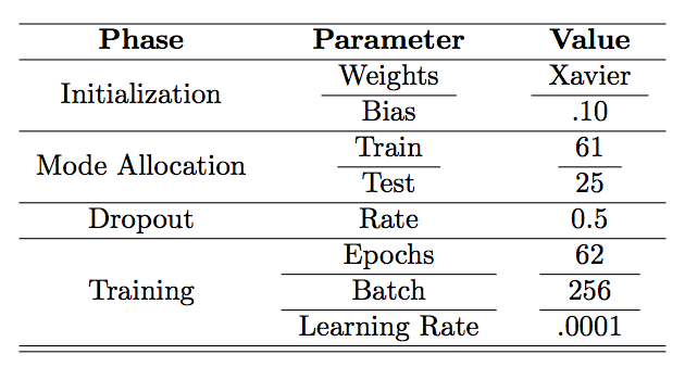
The 7-layer CNN was developed using the MatConvNet deep learning platform4. The proposed CNN utilized convolutional (3x3 kernels), pooling, dropout, and loss layers as shown in Figure 1. We used the weight initialization method proposed by Glorot and Bengio5. For non-linear activation, rectified linear units (ReLU)6 were used. Dropout7 was used on convolutional and fully connected layers. L2 regularization was used on kernel weights. We minimized the binary log-loss when classes are defined "not bone" and "bone" using stochastic gradient descent with momentum as an optimization algorithm8. We extracted axial, coronal, and sagittal 32x32 patches centered at each voxel to generate a patch based dataset reflecting 2.5D representation9 and using 2D convolution kernels in CNN. Training parameters are outlined in Table 1.
High resolution MR hip microarchitecture FLASH images (TR/TE=31/4.92ms; flip angle, 25°; in-plane voxel size, 0.234 x 0.234 mm; section thickness, 1.5mm; number of coronal sections, 60; acquisition time, 25 minutes 30 seconds; bandwidth, 200Hz/pixel) from n=61 volunteers were used for training the CNN. Images were obtained using commercial 3T MR scanner (Skyra, Siemens, Erlangen) with a 26-element radiofrequency coil setup (18-element Siemens commercial flexible array and 8-elements from the Siemens commercial spine array). Trained CNN was tested on 25 subjects whose data was not used in training to identify the model.
We performed post-processing on the segmentation results to remove small clusters of misclassified bone regions and adjust for prior knowledge. We imposed volumetric constraints by removing clusters smaller than predefined thresholds. We also performed basic morphological operations, such as filling holes and opening.
Results
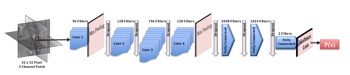
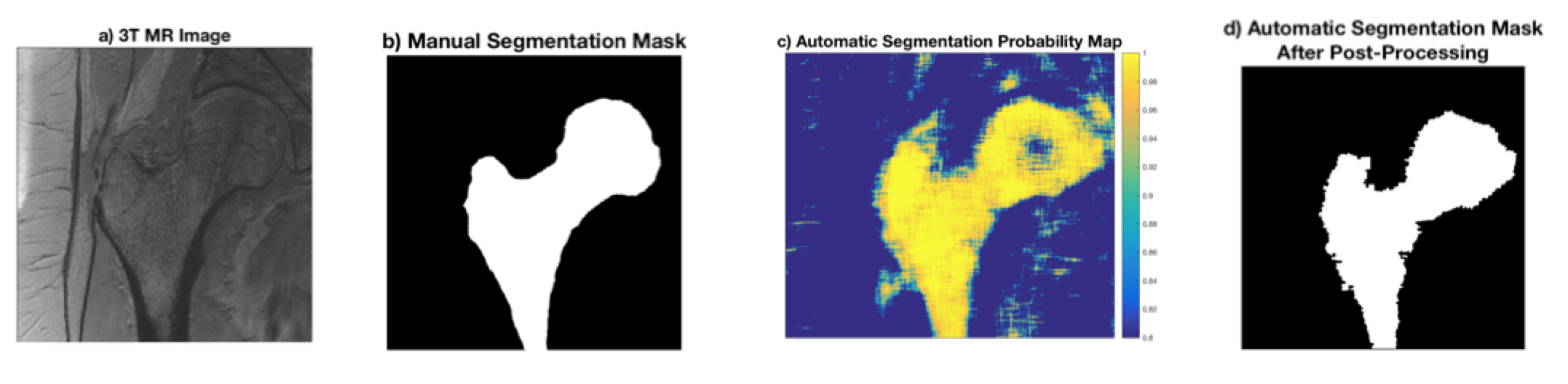
Figure 2 represents the original axial MR image (2a), the ground-truth segmentation (2b), a probability map output of the network (2c), and the network output projection after post-processing (2d). Receiver operator characteristics (ROC) on the probability maps across 29 slices in 25 cases were used to obtain the optimal cutoff value of .9266 for separating bone/non-bone regions (Figure 3). AUC, sensitivity, and specificity values from test cases were 0.933, 0.611, and 0.971, respectively with the proposed model.
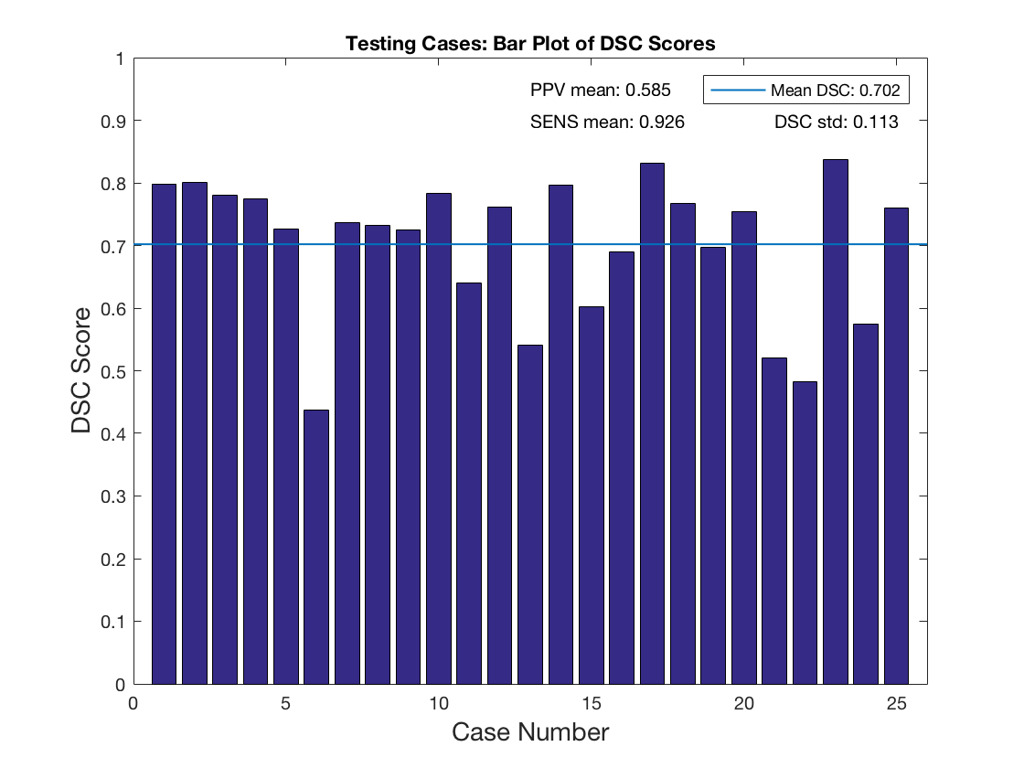
Figure 4 shows DSC scores case-wise with overall DSC score across all cases superposed. The proposed algorithm has a mean DSC score of 70.2±11.3% from 25 test cases. Overall positive predictive value (PPV) and sensitivity scores were 58.5±15.0% and 92.6±4.70%, respectively.
We performed manual fine-tuning on CNN segmentation results to investigate if the CNN model had reduced the time required for manual segmentation. Manual fine-tuning on CNN segmentations resulted in 40% decrease in total segmentation time compared to manual segmentation alone (8 minutes versus 14 minutes 30 seconds).
Discussion and Conclusions
We implemented and tested a CNN for automatic proximal femur image segmentation. High ROC specificity scores indicate the network's efficacy in predicting non-bone elements. Moderate ROC sensitivity scores suggest that errors are from false negative results, which agrees with prior expectation since non-bone elements comprised the majority of training data. In future implementations, we will incorporate imbalanced class information directly into the loss function during training, improving the ROC sensitivity score and segmentation fidelity. We plan to improve the model implementation by incorporating postprocessing by introducing conditional random field (CRF) at the output of the CNN.
Both peak and average fidelity scores are aligned with those produced by state-of-the-art leaders in the field,2,10 reinforcing that deep learning is a proficient proximal femur segmentation option. Mean DSC similarity scores can be further improved above the 70.2% mean when removing outlier cases below DSC=50% (2 cases). Trends in low DSC score cases will be further analyzed to determine inefficiencies in the CNN deployment.
Acknowledgements
This work was supported in part by NIH R01 AR066008 and was performed under the rubric of the Center for Advanced Imaging Innovation and Research (CAI2R, www.cai2r.net), a NIBIB Biomedical Technology Resource Center (NIH P41 EB017183)References
1. Link, T. (2012). Osteoporosis imaging: State of the art and advanced imaging. Radiology, 263(1), 3-17.
2. Pereira, S., Pinto, A., Alves, V., & Silva, C. (2016). Brain Tumor Segmentation Using Convolutional Neural Networks in MRI Images. Medical Imaging, IEEE Transactions on, 35(5), 1240-1251.
3. Prasoon, A., Petersen, K., Igel, C., Lauze, F., Dam, E., Nielsen, M. (2013). Deep feature learning for knee cartilage segmentation using a triplanar convolutional neural network. Medical Image Computing and Computer-assisted Intervention : MICCAI ... International Conference on Medical Image Computing and Computer-Assisted Intervention, 16(Pt 2), 246-53.
4. "MatConvNet - Convolutional Neural Networks for MATLAB", A. Vedaldi and K. Lenc, Proc. of the ACM Int. Conf. on Multimedia, 2015.
5. Glorot, X. & Bengio, Y. Understanding the difficulty of training deep feedforward neural networks. Aistats 9, 249–256 (2010).
6. Nair, V. & Hinton, G. E. Rectified Linear Units Improve Restricted Boltzmann Machines. Proc. 27th Int. Conf. Mach. Learn. 807–814 (2010). doi:10.1.1.165.6419
7. Srivastava, N., Hinton, G. E., Krizhevsky, A., Sutskever, I. & Salakhutdinov, R. Dropout?: A Simple Way to Prevent Neural Networks from Overfitting. J. Mach. Learn. Res. 15, 1929–1958 (2014).
8. Snoek, J., Larochelle, H. & Adams, R. P. Practical Bayesian Optimization of Machine Learning Algorithms. Adv. Neural Inf. Process. Syst. 25 1–9 (2012). doi:2012arXiv1206.2944S
9. Xu, Yichong, Xiao, Tianjun, Zhang, Jiaxing, Yang, Kuiyuan, & Zhang, Zheng. (2014). Scale-Invariant Convolutional Neural Networks.
10. Roth, H., Lu, L., Farag, A., Shin, H., Liu, J., Turkbey, E., & Summers, R. (2015). DeepOrgan: Multi-level Deep Convolutional Networks for Automated Pancreas Segmentation.
Figures