3976
Deep network training based sparsity model for reconstruction1Electrical Engineering, University of California, Los Angeles, Los Angeles, CA, United States, 2Radiology, University of California, Los Angeles, Los Angeles, CA, United States, 3Skolkovo Institute of Science and Technology, Moscow, Russian Federation
Synopsis
One challenge for MR reconstruction is to heuristically select the appropriate regularizer for the optimization problem. This abstract proposes a novel deep learning based reconstruction approach for accelerated MR imaging. With the training using clinical MR images and their retrospectively undersampled noisy images, this algorithm learns the specific parameters of a general regularizer for the optimization problem, and uses this regularizer in the iterative reconstruction to achieves high image quality with high acceleration factors.
Introduction
In recent years, Parallel imaging is combined with compressed sensing for accelerated MR reconstruction1. It requires heuristic selection of underlying regularizer based on the reconstruction sequence and image type, such as total variation2 or wavelet3. Iterative soft thresholding method with regularization is a well-known method for MRI reconstruction4. Trained nonlinear reaction diffusion model for image sparsifying is novice study5. Inspired by this, this study uses this model to learn a general regularizer so the filter kernels and influence functions are learned instead of manually pre-defined. In this study, we use a variation of convolutional neural network to train the sparsity model offline with clinical MR images. Then we apply the sparsity model to the iterative MR image reconstruction using both retrospectively undersampled DICOM images and scanned undersampled MR k-space data. By combining the iterative soft thresholding reconstruction method with trained sparsity model, we achieved efficient reconstruction with high acceleration factor and high quality image result.Theory and Methods
The reconstruction is the optimization problem
$$\arg\min_x \left \{ \| y - \mathcal{UFPS}x \|^2_2 + \lambda \mathcal{D}(x) \right \},$$
where $$$y$$$ is the acquired undersampled k-space data; $$$x$$$ is the result MR image; $$$\mathcal{F}$$$ is the Fourier transform; $$$\mathcal{U}$$$ is the undersampling mask; $$$\mathcal{S}$$$ is the sensitivity map; $$$\mathcal{P}$$$ is the phase correction; $$$\mathcal{D}$$$ is the sparsifying operator, and $$$\lambda$$$ is its weight. The reconstruction is then solved iteratively to find the real-valued image $$$x$$$. $$$\mathcal{D(x)}$$$ is of the form $$$\mathcal{D}(x) = \sum_{n=1}^{N}\rho(K_ix)_n) = \sum_{n=1}^{N}\sum_{i=1}^{N_k} \rho_i((K_ix)_n)$$$; $$$\rho$$$ is the potential function, and $$$K_i$$$ is the sparse matrix implemented as a convolution of image by filter kernels $$$k_i$$$.
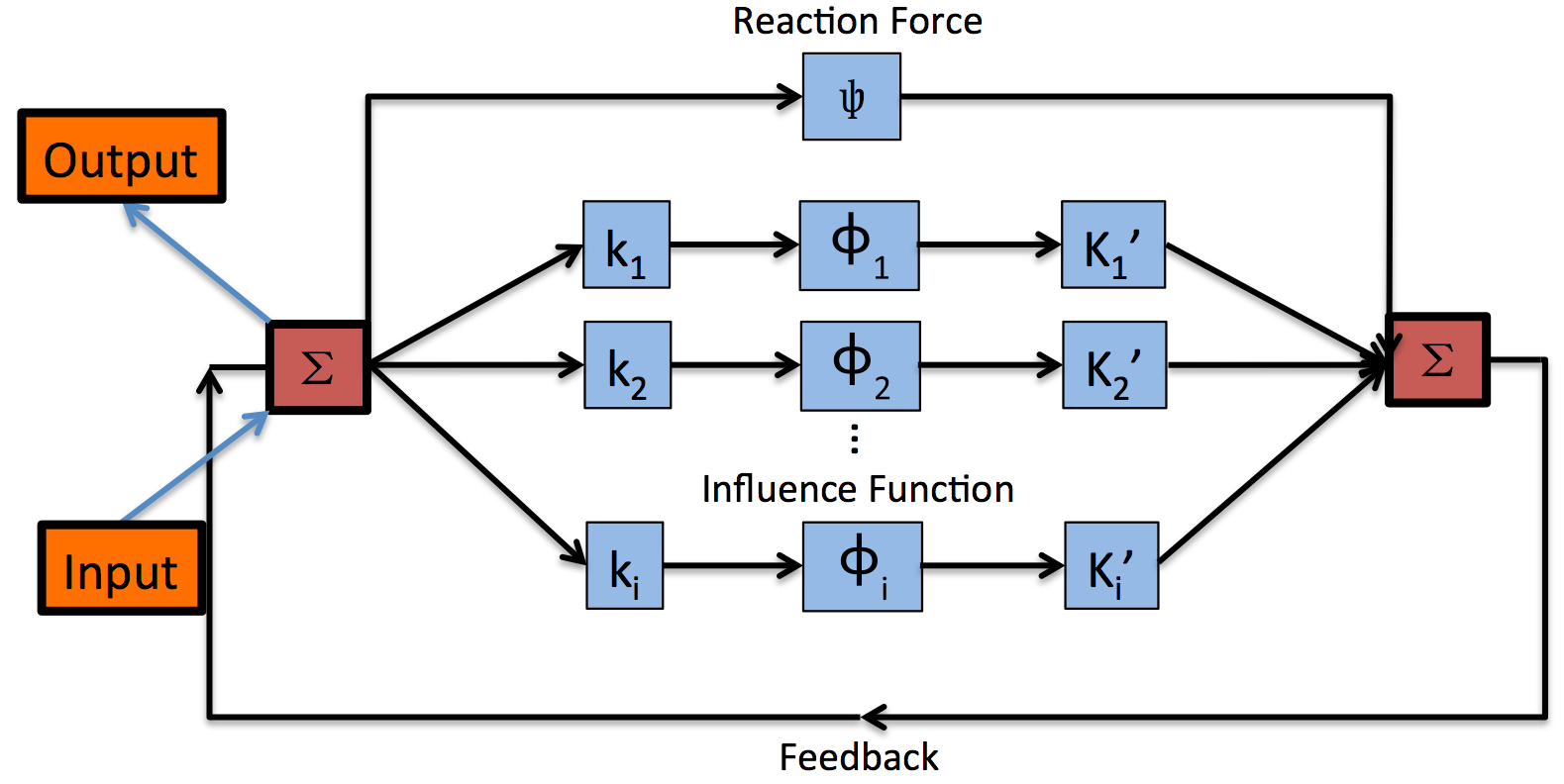
The sparsity model used in this study can be formulated as
$$\frac{u_t-u_{t-1}}{\Delta t} = - \sum_{i=1}^{N_k} K_i^{t \intercal} \phi_i^t (K_i^tu_{t-1}) - \psi(u_{t-1},f),$$
where $$$\phi_i$$$ is the influence functions and in this case the derivative of $$$\rho_i$$$6; $$$u$$$ is the image in column vectors5; $$$\psi$$$ is the reaction force and in this case is $$$\psi(u) = \bigtriangledown_u\mathcal{D}(u)$$$5; $$$f$$$ is the degraded image. $$$\Delta t$$$ is set to 1 and this equation is one step of the gradient descent process5. $$$\lambda$$$, $$$\phi_i$$$ and $$$k_i$$$ are the unknown parameters to be trained5. The training network diagram is shown in Figure 1. Compared to regular convolutional neural network (CNN), this network contains a feedback step, and thus can be viewed as a recurrent network5.
Experiments and Results
Both training and reconstruction are performed in MATLAB 2016a (The MathWorks, Inc., Natick, Massachusetts, USA). The training of a specific acceleration factor is using 100 slices of clinical 3D T1 Vibe fat suppressed liver DICOM images, cropped to 180×180. We use the clinical MR images as clean input and their retrospectively undersampled images as the noisy input. 8 stages of 48 7×7 filters are used, and each training takes about 50 hours.
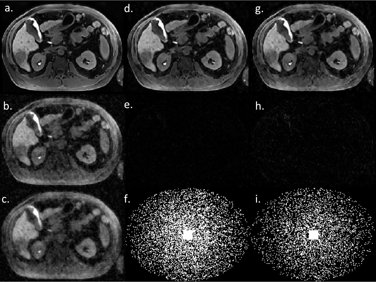
DICOM image reconstruction: DICOM test image is one slice of fat suppressed 3D Vibe image. It is Fourier transformed to k-space and retrospectively undersampled 4.3X and 6.3X to form the single channel test k-spaces. The k-spaces are reconstructed using the 4.3X and 6.3X sparsity model respectively, shown in Figure 2. Since the k-space is transformed from real-valued image, so there are no sensitivity map and phase correction. The step size and the number of iterations are heuristically selected.
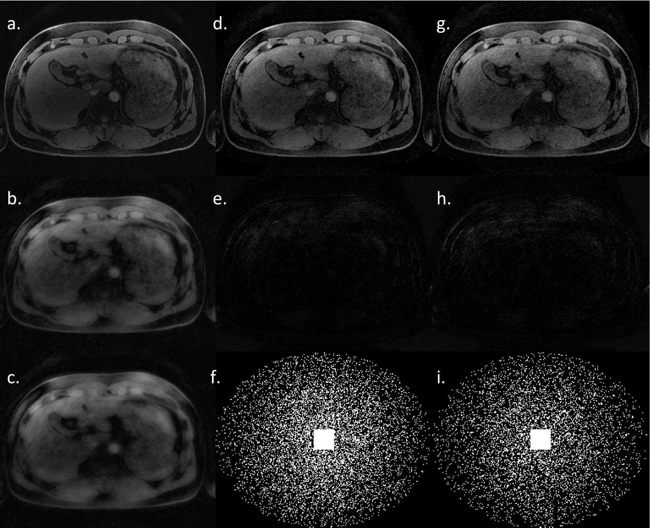
K-space data reconstruction: The test data is one slice of 20-channel k-space, scanned with a volunteer from Siemens 3T Prisma scanner, with 3D T1 Vibe fat suppressed breath-hold sequence. It is then retrospectively undersampled by 6.2X and 8.0X, and reconstructed using 6.2X and 8.0X sparsity model respectively, shown in Figure 3. The sensitivity maps are estimated from undersampled k-space using ecalib function from BART toolbox7. The phase maps for each channel from zero-filled complex images are used for phase correction. The step size and the number of iterations are heuristically selected.
Discussion
In DICOM image reconstruction, our method shows high-fidelity reconstruction result for a high acceleration factors, the lesion in the liver is clearly reconstructed. In K-space data reconstruction, combined with parallel imaging and phase correction, our method can reach a very high number of accelerations with a reasonable image quality. The main source of artifact comes from the inaccuracy of phase correction. The estimated phase from zero-filled image degrades the reconstruction quality, and reconstruction with fully sampled phase correction confirms it.
Conclusion
Our reconstruction method shows promising result, that it can reach good image quality with high acceleration factor. With the trained models from different sets of MR images, it can be used to reconstruct MR images from different sequences and body regions.Acknowledgements
This study is supported by NSF: CCF-1436827.References
1.Lustig, Michael, and John M. Pauly. "SPIRiT: Iterative self-consistent parallel imaging reconstruction from arbitrary k-space." Magnetic resonance in medicine 64.2 (2010): 457-471.
2. Tang, Jie, Brian E. Nett, and Guang-Hong Chen. "Performance comparison between total variation (TV)-based compressed sensing and statistical iterative reconstruction algorithms." Physics in medicine and biology 54.19 (2009): 5781.
3. Lustig, Michael, David Donoho, and John M. Pauly. "Sparse MRI: The application of compressed sensing for rapid MR imaging." Magnetic resonance in medicine 58.6 (2007): 1182-1195.
4. Beck, Amir, and Marc Teboulle. "A fast iterative shrinkage-thresholding algorithm for linear inverse problems." SIAM journal on imaging sciences 2.1 (2009): 183-202.
5. Chen, Yunjin, and Thomas Pock. "Trainable Nonlinear Reaction Diffusion: A Flexible Framework for Fast and Effective Image Restoration." arXiv preprint arXiv:1508.02848 (2015).
6. Black, Michael, et al. "Robust anisotropic diffusion and sharpening of scalar and vector images." Image Processing, 1997. Proceedings., International Conference on. Vol. 1. IEEE, 1997.
7. Martin Uecker, Frank Ong, Jonathan I Tamir, Dara Bahri, Patrick Virtue, Joseph Y Cheng, Tao Zhang, and Michael Lustig, Berkeley Advanced Reconstruction Toolbox, Annual Meeting ISMRM, Toronto 2015, In Proc. Intl. Soc. Mag. Reson. Med. 23:2486
Figures