Introduction

The potential of single-point imaging techniques for the imaging of short $$$T_2^\star$$$ relaxation time systems is applicable to a wide field of applications, such as areas of increased susceptibilities, but it is still limited by the long scan time, demanding strong undersampling to approach clinically acceptable scan times. The SPRITE sequence (single-point ramped imaging with $$$T_1$$$ enhancement) has been successfully introduced and tested for the scan time reducing use at gas Imaging¹ and in vivo for animal Imaging². Impairments can only be addressed by the application of advanced reconstruction techniques like Compressed Sensing or GRAPPA, whereas the first one is introduced in this contribution, which relies on an optimized acquisition trajectory with noise-like PSF. Quasi-random trajectories provide minor coupling of coefficients in the transformed domain, leading to qualifying image optimizations, by also overcoming reconstruction issues using the method of Dirichlet tessellations.

Methods

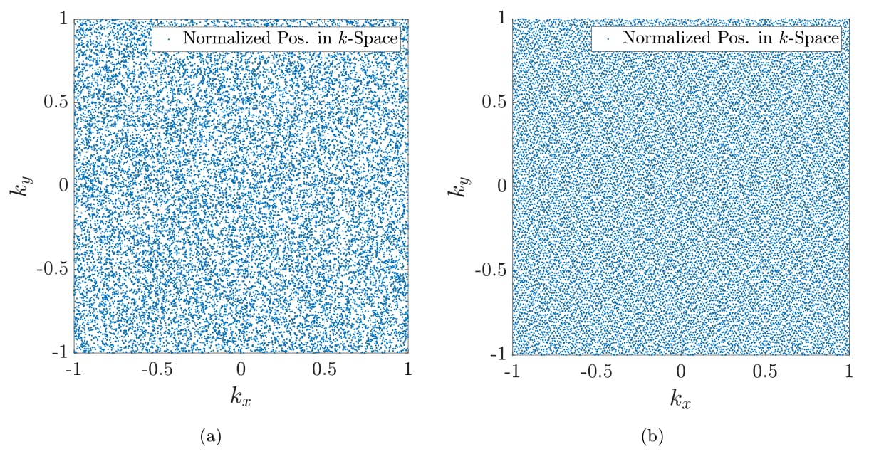
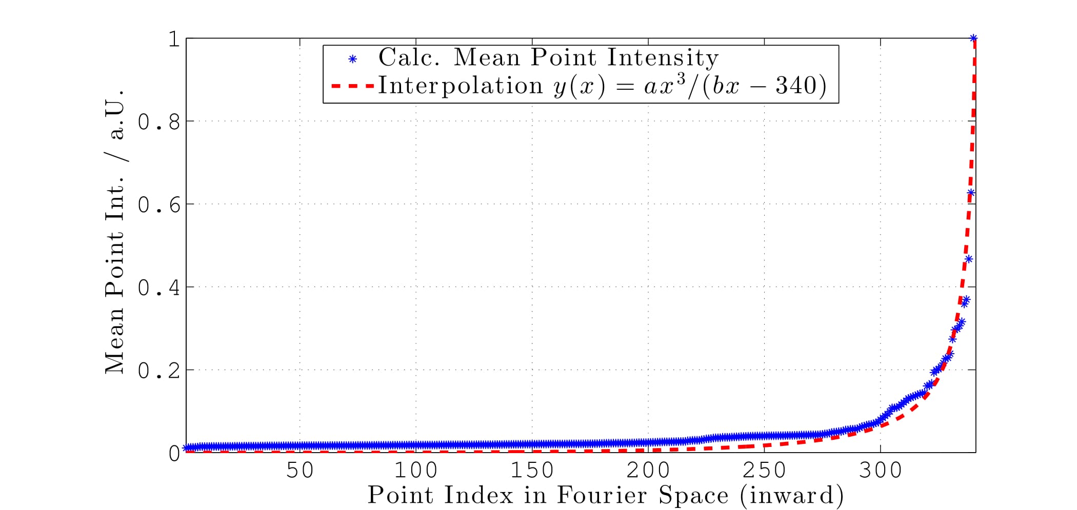
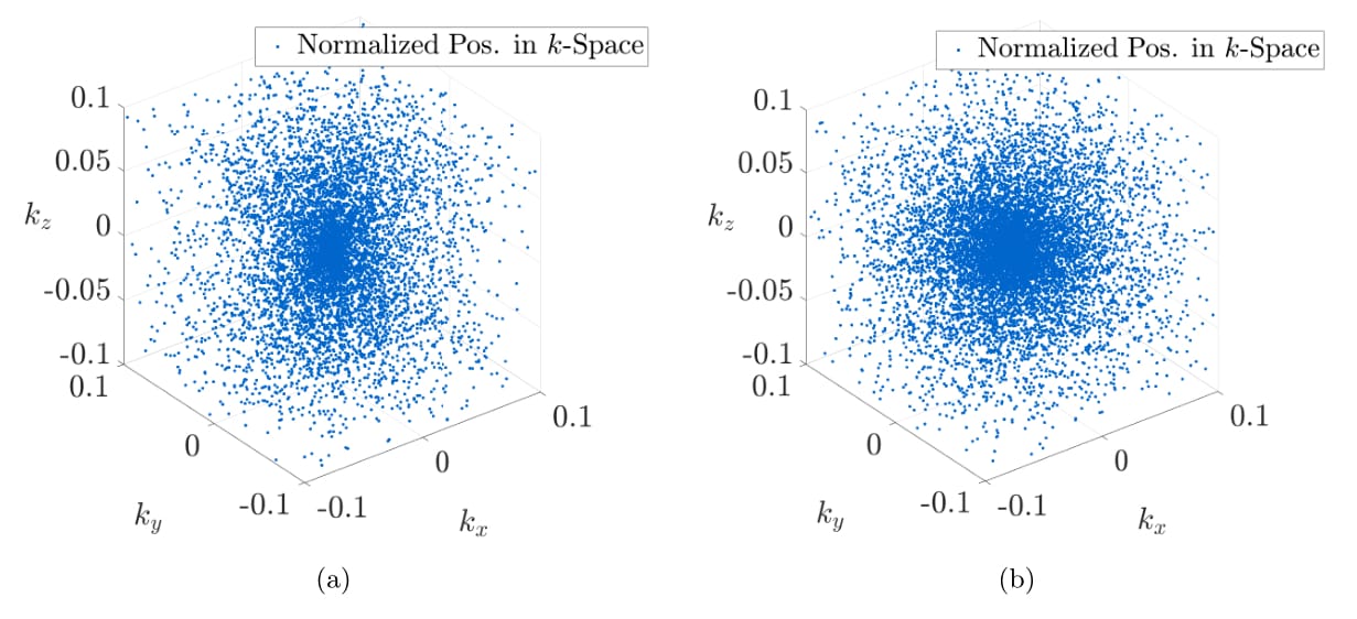
We created a trajectory, consisting of three-dimensional point-sets, generated using a Sobol base-2 low-discrepancy sequence. In order to generate one set of datapoints, making up one dimension of the final set of $$$N$$$-bit, odd (positive) integers $$$m_i$$$ with $$$0\leq i < N$$$ are chosen. Each integer can be used to calculate a "direction" $$$d_i$$$ with $$$d_i = m_i/2^i$$$. The result of this fraction can be binary expanded such that $$$d_i = 0.c_{i,1}c_{i,2}c_{i,3}...\,$$$. One is now free to choose a polynomial $$$P(x)$$$ within a finite field (binary) of degree $$$n$$$ with coefficients $$$a_i$$$ such that:$$P(x) = x^n + a_1x^{n-1}+a_2x^{n-2}+...+a_{n-1}x^1+1.$$ The obtained coefficients can now be used to calculate each direction vector $$$c_i$$$ via $$c_i = a_1c_{i-1} \oplus a_2c_{i-2} \oplus a_3c_{i-3} \oplus ... \oplus a_{n-1}c_{i-n+1} \oplus c_{i-d} \oplus \{ c_{i-d} \gg n \}$$ in which $$$\oplus$$$ denotes the logical exclusive-or and the last term is right-shifted by $$$n$$$ bits. The sequence of points $$$x_1,x_2,...$$$ is now obtained from the relation $$x_n = i_1c_1 \oplus i_2c_2 \oplus i_3c_3 ...,$$ where $$$i_k$$$ is the $$$k$$$-th digit from the right when $$$i$$$ is written in binary $$$i = (...i_3i_2i_1)_2$$$ representation. Figure 1 displays twenty-thousand points, generated using Matlab's rand()-function, and using the previously described low-discrepancy method within a normalized two-dimensional $$$k$$$-space. Furthermore, if several reconstructed MR images with an equal reconstruction matrix size are Fourier transformed into the frequency domain, and the point intensity is evaluated in centre-out fashion of all possible spokes of all images, then a course as depicted in figure 2 is obtained. The mean point intensities can be well interpolated using the same model as for the mentioned radial centre-out density distribution. It is therefore advantageous to create a quadratic density modulation over the Sobol base-2 point-set. This is accomplished by projecting each $$$n$$$-th point of the Sobol point-set sequence around the centre of $$$k$$$-space using a quadratic density distribution. Nevertheless, the new angular position still follows a random behaviour and will therefore lead to an effect known as "point clumping" i.e. a stretching of the point distribution along one spatial axis, as shown in figure 3a for the real three-dimensional case, which was solved using adopted transformations.The discrepancy of the sequences is compared using the diaphony, which is closely connected to the star-discrepancy, but computable for large datasets within an acceptable amount of time. The diaphony $$$F_N(X)$$$ of the first $$$N$$$ Points $$$x_1,x_2,...,x_N$$$ of a one-dimensional point-set $$$X$$$ is defined as $$F_N(X) := \left( 2\pi^2 \int\limits_0^1 \int\limits_0^1{|E([\alpha,\beta),N,X)|^2 \text{d}\alpha\text{d}\beta} \right )^{1/2}$$ with $$$[\alpha,\beta) \subseteq I = [0,1)$$$ and $$$E([\alpha,\beta),N,X) = A([\alpha,\beta),N,X)-(\beta-\alpha)N$$$. $$$A$$$ denotes the number of indices $$$1\leq i \leq N$$$ for which $$$\{ x_i\} \in [\alpha,\beta)$$$.

Results and Discussion

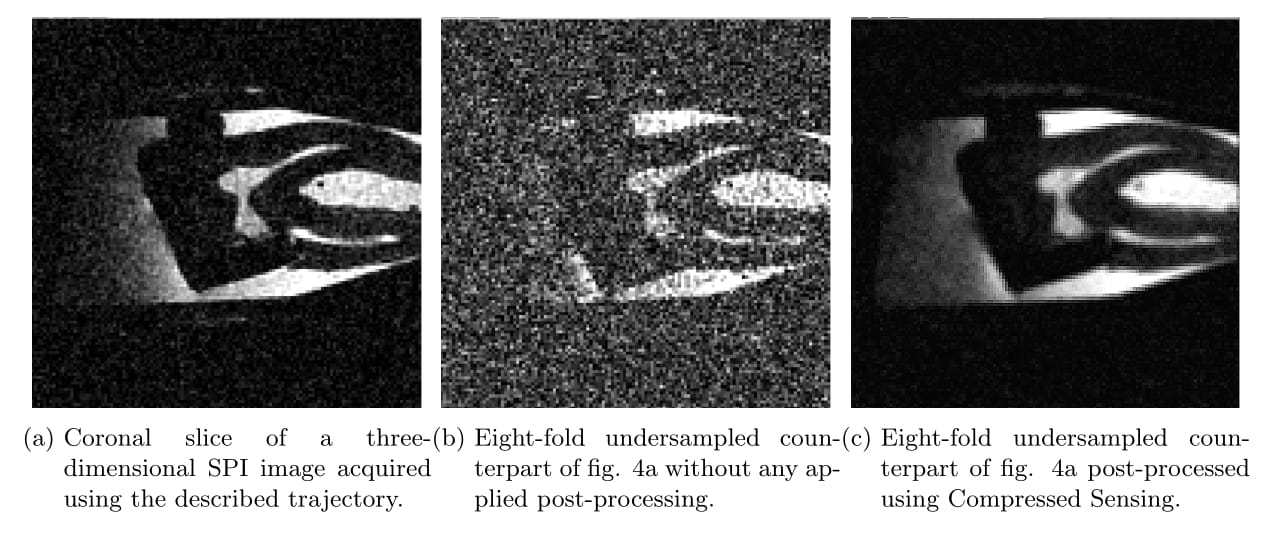
The diaphony of the trajectory, displayed in fig. 3a is given by $$$F_\text{rnd} = 7.57\cdot 10^{-3}$$$, while the diaphony of fig. 3b is calculated to $$$F_\text{sob} = 1.4\cdot 10^{-4}$$$ with $$$F_\text{rnd}/F_\text{sob} \approx 54$$$. This provides a serious optimization in point distribution over the complete space. Figure 4 shows a reconstructed tooth image, using known³ reconstruction methods, acquired with the described trajectory aside with its eight-fold undersampled counterpart and once post-processed using Compressed Sensing. All images were acquired using a Bruker BioSpec 117/16 USR preclinical MR system. The metal containing tooth crown does not show any susceptibility artefact and therefore remains sharply confined.

Conclusion

The presented trajectory provides highly useful undersampling properties (random-noise-like) for the combination with Compressed Sensing due to its quasi-random generation algorithm. The sequence does not require any intrinsic oversampling e.g. by a factor of $$$\pi/2$$$ which makes an image as shown in figure 4c acquirable within less than 6 min. Susceptibility and chemical shift artefacts are successfully suppressed, leading to a wide range of application fields.

Acknowledgements

No acknowledgement found.