3962

In-vivo Validation of MR-STAT: Simultaneous Signal Localization and Quantification of Tissue Parameters on a 3T Clinical MR-System

Oscar van der Heide¹, Alessandro Sbrizzi¹, Anna Kruseman¹, Martijn Cloos², Peter Luijten¹, and Nico van den Berg¹

¹UMC Utrecht, Utrecht, Netherlands, ²NYU School of Medicine, New York, United States

Synopsis

MR-STAT is a framework for obtaining quantitative parameter maps from a single short scan. It is based on a time domain model. Large numerical inversion problems are solved to simultaneously localize signal and estimate tissue parameters. In this work we demonstrate the first experimental in-vivo results obtained with a clinical MR system.

Purpose

MR-Fingerprinting (MRF) is a new multi-parametric quantitative MR technique that uses data from a single short scan following a two-step procedure.¹First a series of highly undersampled images is reconstructed. Then the observed signal is matched to a pre-computed dictionary of spin evolutions. In MRF, incoherent aliasing artifacts in the images add a large stochastic component to the measured signal. The previously introduced MR-STAT method eliminates this stochastic component by treating the entire problem (signal localization and parameter estimation) as one large-scale inversion problem.^2,3 Here we present the first in-vivo MR-STAT results using a Cartesian 2D gradient-balanced sequence on a clinical MR-system.

Theory

The MR time-domain signal $$$S$$$ is modeled using Faraday's Law as $$S(\alpha,t)=\int_{V}B_{1}^{-}(\vec{r})m_{xy}(\alpha(\vec{r}),t)d\vec{r},$$ where $$$B_{1}^{-}$$$ is the receive field and $$$m_{xy}$$$ is the transverse magnetization. The time evolution of $$$m_{xy}$$$ is described by the Bloch equation and depends on the underlying tissue parameters, grouped together in $$$\alpha(\vec{r}):=\left(T_{1}(\vec{r}),T_{2}(\vec{r}),\Delta B_{0}(\vec{r}),B_{1}^{+}(\vec{r}),\rho(\vec{r}),\ldots\right)$$$). Let $$$d$$$ represent the actual measured time-domain signal. The central idea of MR-STAT is to obtain the parameter maps $$$\hat{\alpha}$$$ by solving the non-linear inversion problem $$\hat{\alpha}=\text{argmin}_{\alpha}\int_{[0,T]}\left|d(t)-S(\alpha,t)\right|^{2}dt,$$ where $$$T$$$ is the total sequence length. It is assumed here that the pulse sequence uniquely encodes the parameter maps into the signal. Since MR-STAT is based on a time-domain model, the signal localization and estimation of tissue parameters are performed simultaneously. Obtaining solutions to the resulting large-scale inversion problem requires advanced numerical algorithms. Accuracy of the $$$T_{1},T_{2},B_{0},B_{1}^{+},\rho,\ldots$$$ reconstructions is monitored through the difference between measured and simulated signal. The parameter maps are deemed accurate if the residual is in the thermal noise level. Precision of the reconstructions can be estimated through standard deviation maps obtained from MR-STAT.

Methods

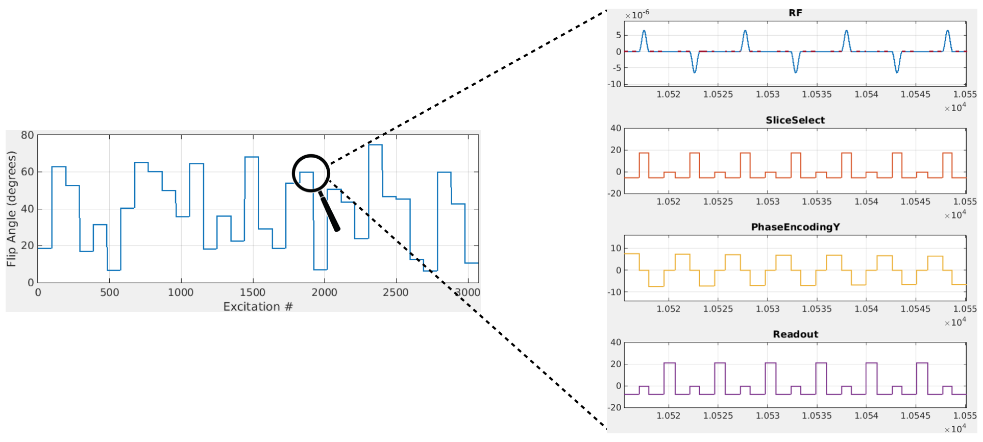
A 2D balanced gradient-echo sequence is used. Spatial encoding is performed using a Cartesian readout scheme. A total of 32 full k-spaces are acquired, each one with a different flip angle and no waiting times. The flip-angles are chosen randomly between $$$5^{\circ}$$$ and $$$75^{\circ}$$$ (Fig. 1). The excitation phases alternate between $$$0^{\circ}$$$ and $$$180^{\circ}$$$. The sequence is preceded by an inversion pulse.

MR-STAT was implemented on a 3T whole-body MR system (Philips-Ingenia). Single slices are acquired for gadolinium-doped agarose gel-samples and a brain of a volunteer with a 15 channel receive head-coil. Total sequence time was 16s.

Sequence parameters were imported into MATLAB. A 1D Fourier transform was applied along the readout direction to decouple the problem into smaller subproblems. These were solved in parallel on a local High Performance Computing (HPC) facility using a MATLAB implementation of VarPro⁴ and a Bloch simulator⁵. The reconstruction time (= longest job) was 12 minutes in both cases.

Our model does not require knowledge of RF transmit fields, off-resonance and/or proton density. The slice profile is included in the model. In this work we reconstruct $$$T_{1}$$$ and $$$T_{2}$$$. A 5-minute interleaved inversion-recovery and multi spin-echo sequence that comes with our MR-system was used to obtain $$$T_{1}$$$ and $$$T_{2}$$$ values for the phantoms as a reference.

Results

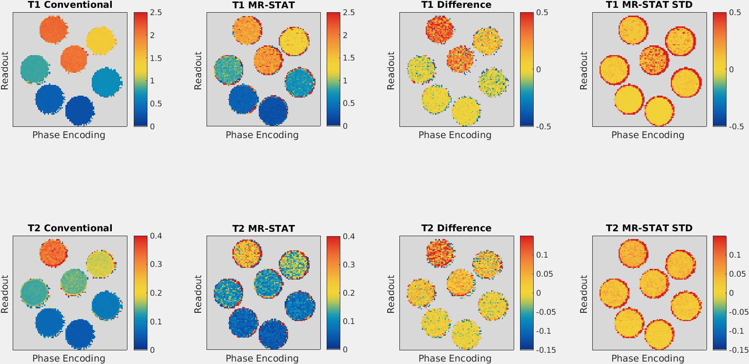
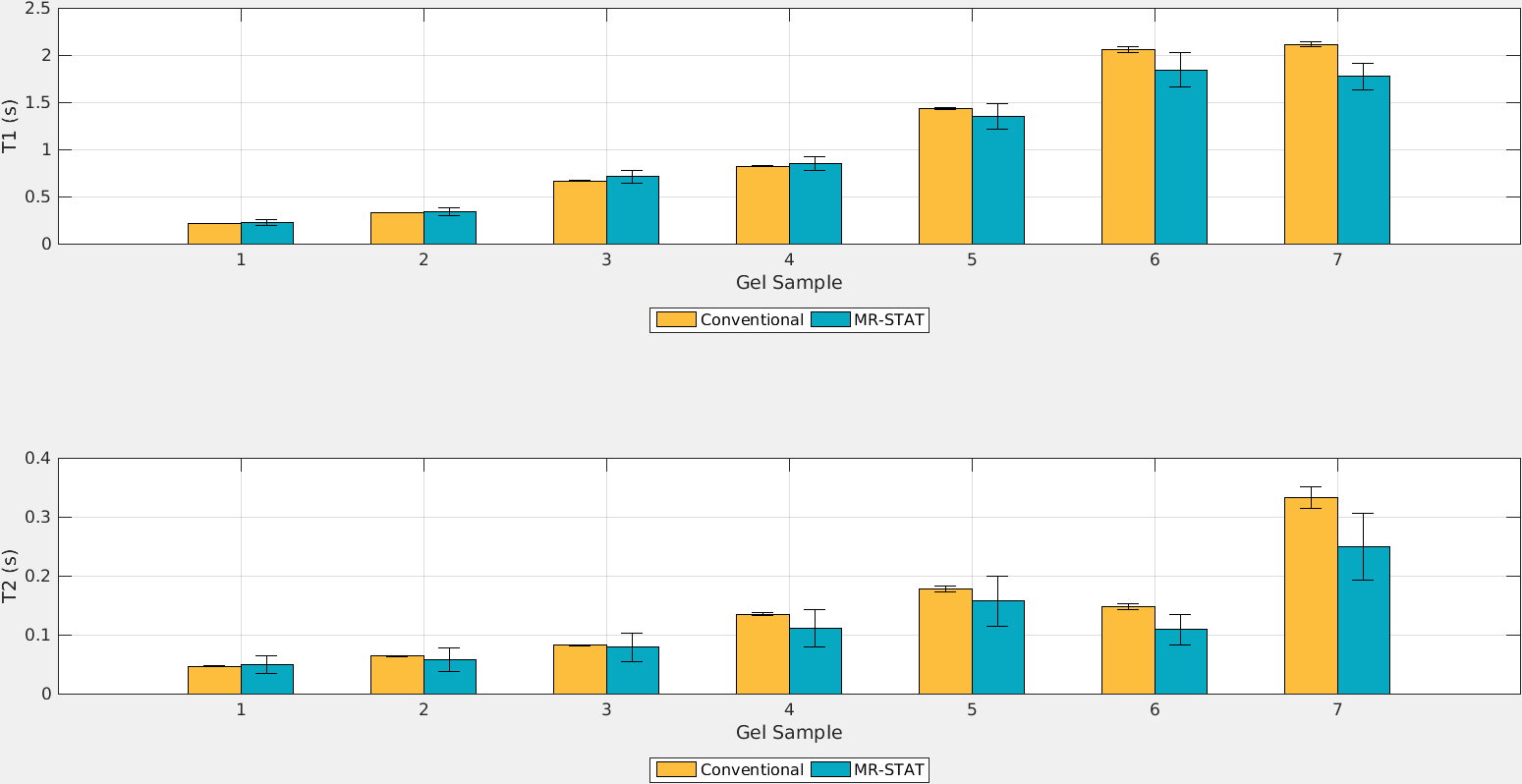
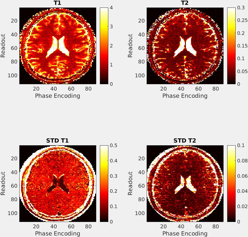
In Fig. 2 the reconstructed $$$T_{1}$$$ and $$$T_{2}$$$ and standard deviation maps obtained with MR-STAT are shown for the gel samples. The reference and difference maps are also shown. In Fig. 3 the mean values of the individual tubes are compared. For the samples with low $$$T_{1}$$$ and $$$T_{2}$$$, the values found with MR-STAT are in good agreement with those found using the conventional method. The $$$T_{1}$$$ and $$$T_{2}$$$ and standard deviation maps from the MR-STAT in-vivo brain scan are reported in Fig. 4.

Discussion

Previous work on MR-STAT was limited to computational proof-of-principle demonstrations. In this work we have successfully applied MR-STAT for the first time on a clinical MR-system. The results show that MR-STAT can simultaneously perform signal localization and parameter estimation using time-domain data from a simple 16s scan.

Unlike MRF, MR-STAT is based on a deterministic process that monitors the accuracy and precision. Instead of relying on a pre-computed dictionary, a large-scale inversion problem is solved. 2D scan's results show that the reconstruction can be performed in reasonable times on a cluster.

Since Fourier Transform is not applied over the whole k-space (MR-STAT works in the time-domain) there is increased flexibility in sequence design.

Parallel imaging and/or compressed sensing strategies could be implemented to further accelerate scan time and/or increase precision.

Conclusion

We experimentally demonstrated the feasibility of MR-STAT with a 16s 2D gradient-balanced sequence on a 3T clinical MR-system. In both phantom and in-vivo experiments MR-STAT was able to simultaneously localize the signal, quantify the $$$T_{1}$$$ and the $$$T_{2}$$$ of the tissue and estimate the precision of the measurement.

Acknowledgements

This research is funded by the Dutch Technology Foundation, Grant #14125.

References

[1] Ma D. et al, Nature 2013.

[2] Sbrizzi A. et al, ISMRM 2015, p. 3712.

[3] Sbrizzi A. et al, ISMRM 2016, p. 4226.

[4] O’Leary, D.P. & Rust, B.W. Comput Optim Appl (2013) 54: 579.

[5] Hargreaves, B., http://www-mrsrl.stanford.edu/~brian/blochsim.

Figures

Figure 1: Pattern of flip angles used (left) and a few $$$T_{R}'s$$$ of the pulse sequence (right).

Figure 2: $$$T_{1}$$$ and $$$T_{2}$$$ maps (in seconds) for agarose gel samples obtained using MR-STAT (first column), conventional methods (second column)and their difference (third column). The standard deviation maps obtained with MR-STAT are shown in the last column. Scan settings used: $$$T_{R}=5.12ms$$$, $$$T_{E}=2.56ms$$$, matrix size $$$96\times96$$$, voxel size $$$1mm\times1mm$$$, slice thickness $$$3mm$$$, total scan time $$$16s$$$.

Figure 3: Bar graph of mean $$$T_{1}$$$ (top) and $$$T_{2}$$$ (bottom) values (in seconds) per gel sample obtained using MR-STAT and conventional methods. Standard deviations are also shown. The scan time for the conventional method was more than 5 minutes while the scan time for MR-STAT was only 16 seconds.

Figure 4: $$$T_{1}$$$ and $$$T_{2}$$$ and standard deviation maps (in seconds) for a human brain obtained with MR-STAT. Scan settings used: $$$T_{R}=5.56ms$$$, $$$T_{E}=2.78ms$$$, matrix size $$$112\times88$$$, voxel size $$$1.8mm\times1.8mm$$$, slice thickness $$$3mm$$$, total scan time $$$16s$$$

Proc. Intl. Soc. Mag. Reson. Med. 25 (2017)

3962