Synopsis

It is well known that the bSSFP signal is highly dependent on the precession frequency off-resonance value at each pixel. The bSSFP signal can be modeled as an ellipse in the complex plane that rotates about the origin, with the degree of rotation depending on the regional off-resonance value. If a specific point on the axis of the ellipse could be localized, the phase of that point could be used to produce a field map. Xiang and Hoff came up with a geometric solution (GS) which removes banding artifacts by estimating a consistent cross point within the ellipse.

Purpose:

Methods:

The bSSFP signal can be written as

$$I(\theta)=M \frac{1-E_2e^{i\theta}}{1-b\cos\theta} e^\frac{-i\beta}{2} e^\frac{-TE}{T_2} \label{eq:1} \\M= \frac{M_0(1-E_1)\sin\alpha}{1-E_1\cos\alpha-E_2^2(E_1-\cos\alpha)}\\b=\frac{E_2(1-E_1)(1+\cos\alpha}{(1-E_1\cos\alpha-E_2^2(E_1-\cos\alpha)}\\E_1=e^\frac{-TR}{T1}, E_2=e^\frac{-TR}{T2}$$

where M0 is the base signal, α is the flip angle, β is the free precession per TR, and θ=2πβ*TR. As a result, the complex estimate of M has a phase that is half the angular free precession per TR, from which it is straightforward to derive a field map by first applying a phase-unwrapping step followed by mapping of free precession per TR to off-resonance.

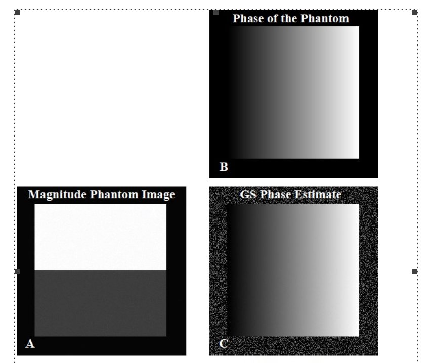
Simulations: A simulated phantom was created with two representative tissues: T1/T2= 300/85 ms (similar to fat) for Tissue 1 and T1/T2= 1200/30 ms (similar to cartilage) for Tissue 2, and free precession per TR values varying from 0 to 4π across both tissues. Other simulated parameters were TR/TE=10/5ms, a=30°, and a base SNR for fat of 30. Four bSSFP images were simulated with phase-cycle increments of 0, π/2, π, and 3π/2. These phase-cycles were then combined using GS, and the phases of the estimates were compared to the simulated actual phase.

Phantom and In-Vivo Experiments: A uniform phantom and normal volunteer were scanned on a 3T Siemens Tim Trio using a 12-channel head coil. A set of four phase-cycles were acquired with increments of 0, π/2, π, and 3π/2. Other parameters included TR/TE=10/5ms, a=30°, FOV=300x300mm, and matrix size=256x256. A GRE field map was taken at the same time for comparison with scan parameters of TR=100 ms and TEs=10 and 5ms, a=30°, FOV=300x300mm, and matrix size=265x256.

Phase unwrapping was performed after reconstructions to compare the two methods. We used the scheme outlined in ⁴.

Results

Simulations: Figure 1 shows the phase maps resulting from the GS and the simulated actual ellipse phase. They are in excellent agreement.

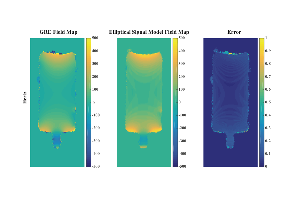
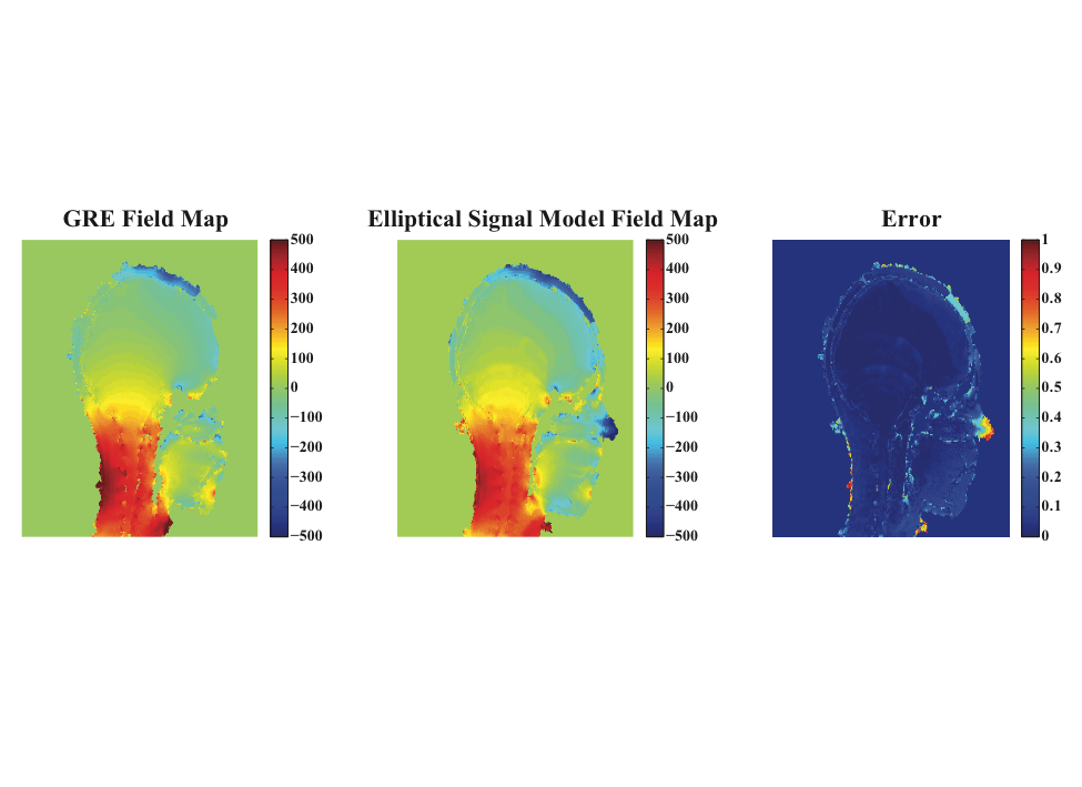
Phantom and In-Vivo Experiments: Figure 2 shows phase maps of a uniform phantom and Figure 3 shows a normal brain using the standard GRE method compared to bSSFP using the GS. Both phantom and in vivo experiments show excellent agreement between the standard GRE method and the GS method.

Accurate field maps can be directly derived from sets of four or more phase-cycled bSSFP images, which are often acquired already to eliminate bSSFP banding artifacts.

Acknowledgements

References

[1] Freeman R, Hill H. Phase and intensity anomalies in fourier transform NMR. J Magn Reson 1971;4:366–383. Q. S.

[2]Xiang and M. N. Hoff, “Banding artifact removal for bSSFP imaging with an elliptical signal model,” Magn. Reson. Med., vol. 71, no. 3, pp. 927–933, 2014.

[3]Hoff and Xiang, “Correcting bSSFP Distortion near Metals with Geometric Solution Phase,” Proc. ISMRM 2013

[4]Spottiswoode, Bruce S., et al. "Tracking myocardial motion from cine DENSE images using spatiotemporal phase unwrapping and temporal fitting." IEEE Transactions on medical imaging 26.1 (2007): 15-30.