3902
Limitations of NMR Field Cameras for B0 Field Monitoring1MPI for Biological Cybernetics, Tuebingen, Germany, 2IMPRS for Cognitive and Systems Neuroscience, Eberhard University of Tuebingen, Tuebingen, Germany, 3Institute of Physics, Ernst-Moritz-Arndt University Greifswald, Greifswald, Germany
Synopsis
We compare the fields measured by a field camera to the fields obtained from B0 mapping at 9.4T. The B0 maps have higher spatial resolution and are therefore taken as a benchmark. We analyse the loss of spatial fidelity due to the lower spatial samples of the field camera and compare two different field probe position calibration and optimisation methods that would help alleviate the problem of discrepancies between field monitoring and field mapping.
Introduction
Field monitoring can be used to correct geometric distortions in MR images, detect frequency shifts, reduce eddy currents, calibrate shim and gradient systems and for real time field stabilization1-5. There are two ways that the B0 field can be monitored. Firstly, using B0 mapping sequences which include full B0 map or projection-based methods6, or secondly, using NMR field cameras1. The former methods require scan time and must be implemented in a sequence and have a higher spatial resolution. The latter method can function independently of the MRI scanner and thus simultaneously with MRI sequences and have a higher temporal resolution, however, the spatial resolution is very low1-2. So far, these two methods have been used for different applications but the real limitations of the trade-off between spatial and temporal resolution have not been previously examined.
In this work, we compare the fields measured by a field camera to the fields obtained from B0 mapping at 9.4T. The B0 maps have higher spatial resolution and are therefore taken as a benchmark. We analyse the loss of spatial fidelity due to the lower spatial samples of the field camera and compare two different field probe position calibration and optimisation methods that would help alleviate the problem of discrepancies between field monitoring and field mapping.
Methods
A 9.4T Siemens whole-body human MRI scanner (Erlangen, Germany) was used. Different B0 fields were generated using an insert shim from Resonance Research Inc. (Billerica, MA) with 28 channels that included 0th, 2nd, 3rd and 4th degree spherical harmonic terms.
B0 fields generated by each of the shim coils (applied current of 1.0A) were measured using a 170 mm diameter silicon oil spherical phantom with an in-house 8-channel transceiver coil7. A 2D gradient echo (GRE) B0 mapping sequence with the following parameters was used: resolution = 1.56x1.56 mm; FOV = 200x200 mm; slice thickness = 3 mm; 40 slices (20% distance factor); TR = 1200 ms; TE = 4.00/4.76 ms; read-out bandwidth 1500 Hz/px.
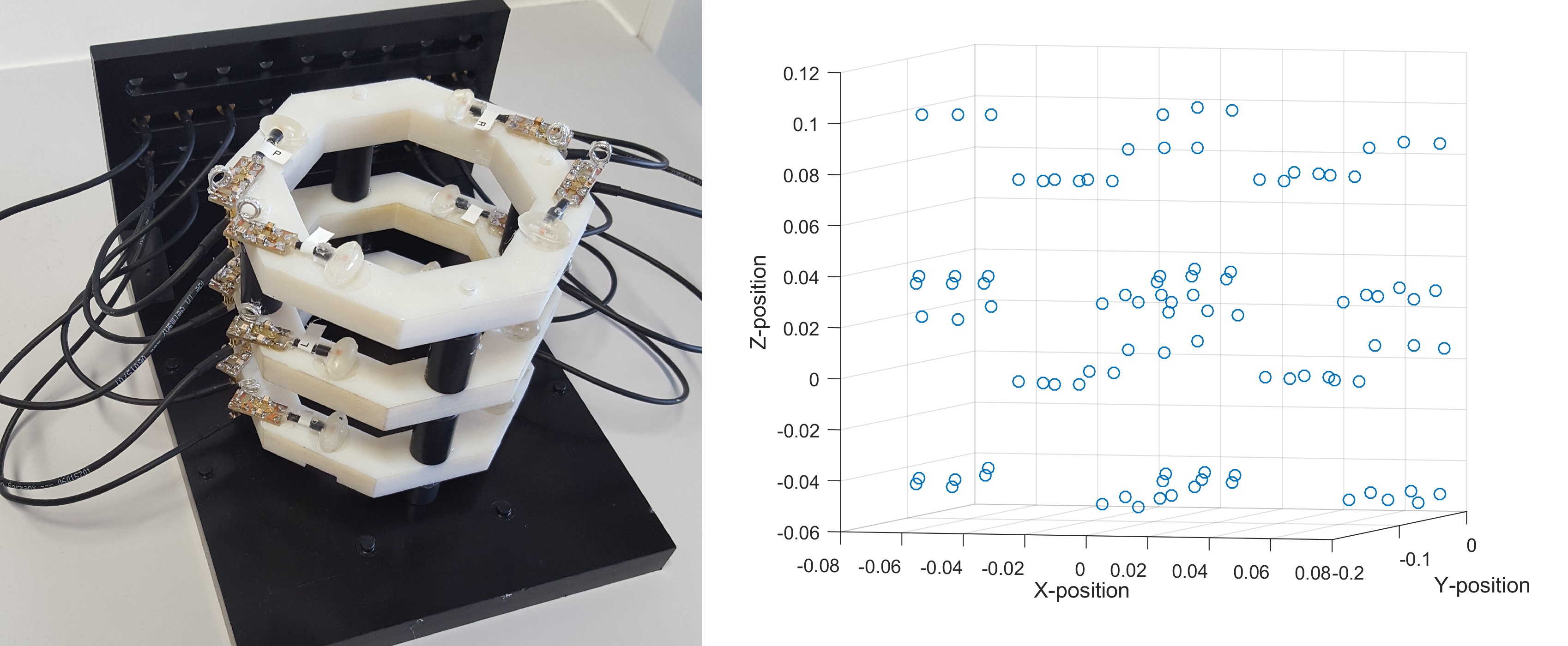
A 1H NMR field camera was built with 12 probes on three layers, i.e. each layer had four probes (Fig. 1). The position of the field camera was calibrated using the gradients: assuming linear gradients (currently used in the literature) and using a constrained optimisation of the measured gradient fields8. The positions of the probes are constrained relative to each other since they are fixed on a rigid body. The optimisation is performed by considering the gradient field nonlinearities.
The field camera was used to measure each of the shim fields (again at 1.0A). This was done for 8 positions of the field camera to increase the number of spatial samples acquired from the field probes. The sample points are shown in Fig. 1.
The fields measured with the field camera were characterised using spherical harmonic decomposition up to the 4th degree. These fields were reconstructed on the FOV of the B0 mapping sequence and compared to the reference fields from the sequence.
Results and Discussion
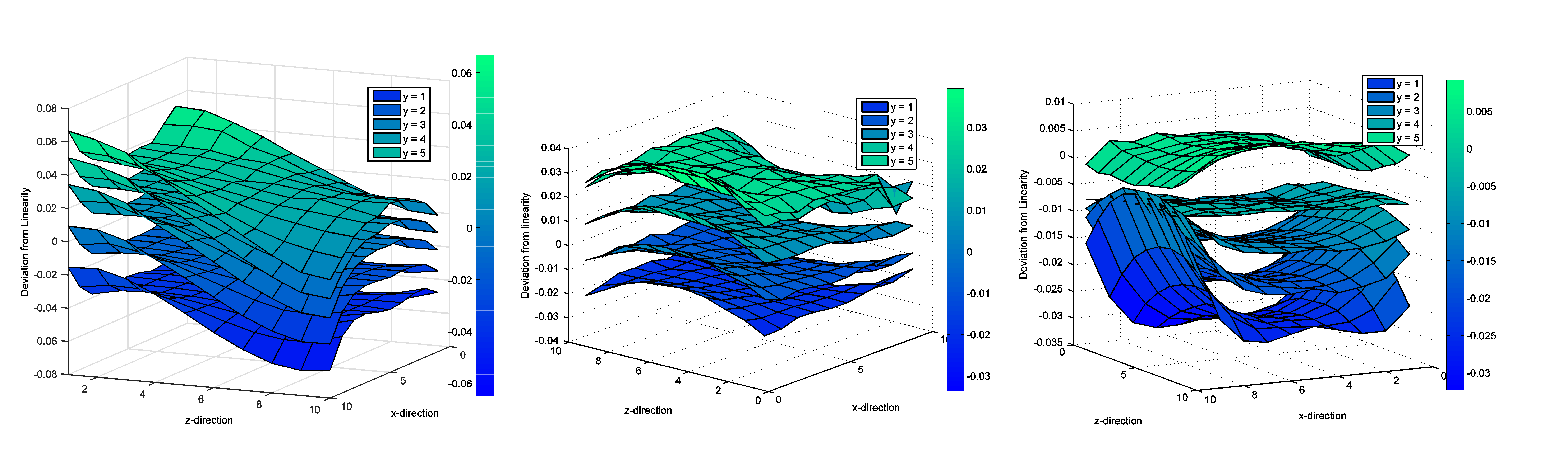
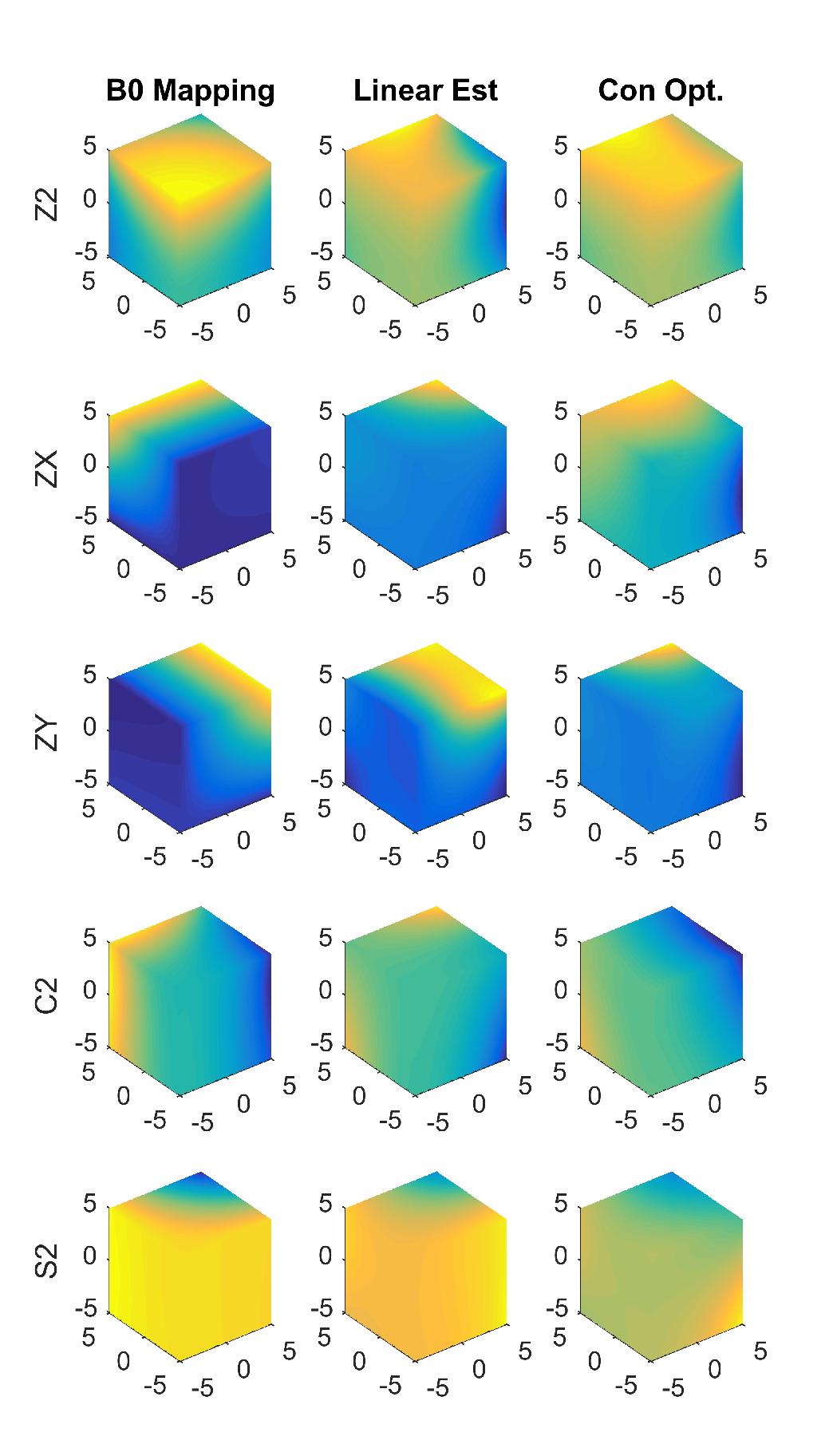
The measured gradient nonlinearities are shown in Fig. 2. The figure shows the deviations from the ideal gradient fields (i.e. for perfect gradients each slice would be flat). The comparison of the B0 mapping to the field probe measurements are shown in Fig. 3 (only 2nd degree shim fields are shown).
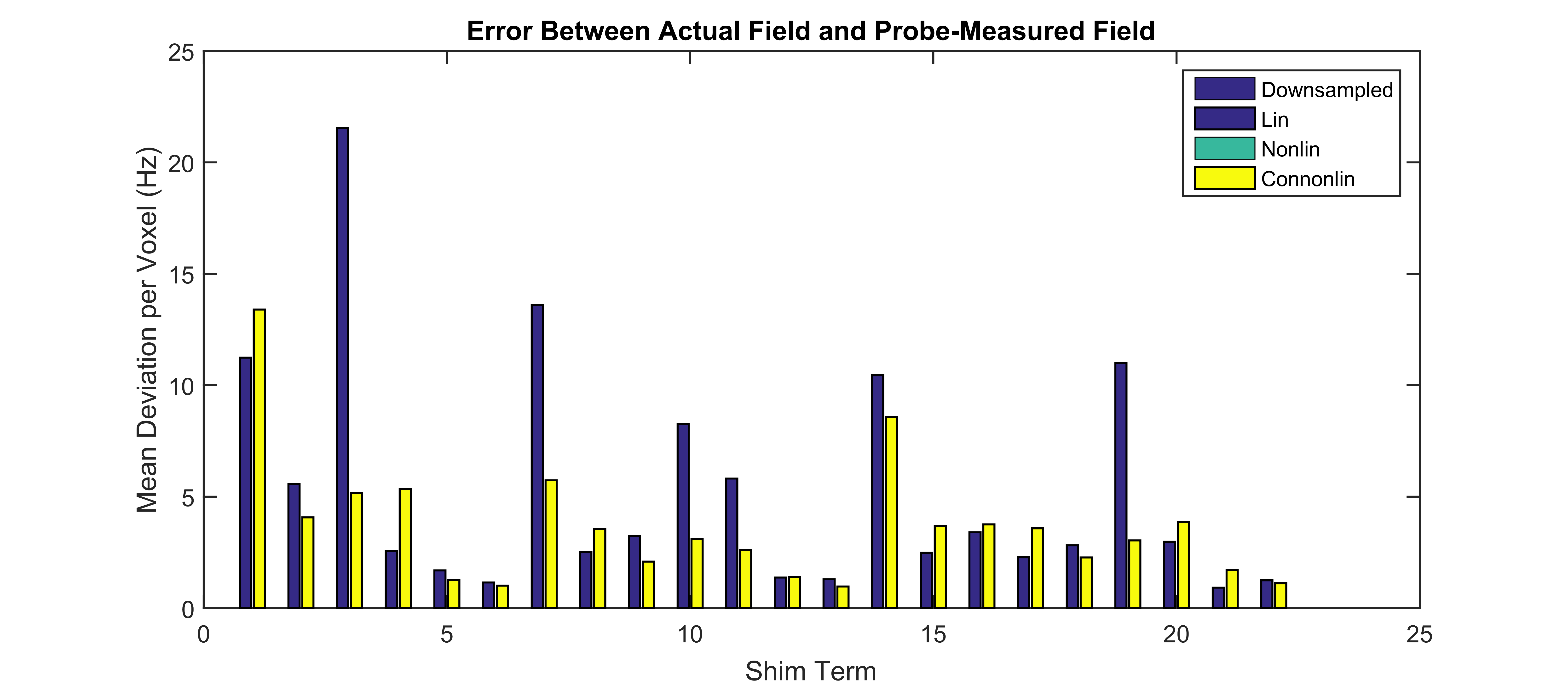
The rmse’s of the fields measured using the B0 mapping and field camera are shown in Fig. 4. This shows that the error introduced by the field camera can be up to a few Hz per voxel.
Although the constrained optimisation position calibration did not always do better than using a linear position calibration, the figure shows that the constrained optimisation is less likely to have large errors (i.e. the median error is lower). The mean error over all shim fields for linear estimation is 5.34 ± 5.28 Hz and for constrained optimisation calibration is 3.70 ± 2.85 Hz.
These findings are also consistent with Anderson et al.9 that show that a 16 probe field camera is not sufficient for 3rd degree B0 shimming.
Conclusion
While NMR field cameras provide a method for high temporal monitoring of the B0 field, this work showed that there is an intrinsic loss due to the low number of spatial sample points. Furthermore, the field camera measurements are dependent on calibration of the positions of the probes which may introduce further errors. The errors can be reduced by using a constrained optimisation calibration of the field camera8.Acknowledgements
No acknowledgement found.References
[1] Barmet C et al. MRM. 2008
[2] De Zanche et al. MRM. 2008
[3] Sipila P et al. MRM. 2011
[4] Wilm B et al. MRM. 2011
[5] Vannesjo et al. MRM. 2015
[6] Shen et al. MRM. 1997
[7] Avdievich et al. NMR Biomed. 2016
[8] Chang P et al. Proc of ISMRM. 2015
[9] Anderson M et al. MRM. 2016
Figures