3867
Total Generalized Variation as a Temporal Regularizer in Compressed Sensing MRI1University of Wisconsin Madison, Madison, WI, United States, 2Waisman Laboratory for Brain Imaging and Behavior, Madison, WI, United States
Synopsis
A novel compressed sensing temporal regularizer, Total Generalized Variation is introduced to enable accelerated temporal imaging. This regularizer eliminates the staircase artifacts typically observed when using a Total Variation regularizer.
Introduction
Quantitative MRI methods including $$$T_1$$$ relaxometry can be very time consuming due to the acquisition of multiple images. Compressed sensing (CS) algorithms with spatial regularizers help to accelerate but have limited benefit due to lack of spatial redundancy. However in inversion recovery (IR) $$$T_1$$$ imaging there is a large amount of redundancy in inversion time direction offering the possibility of CS regularization along that direction. One option would be to use a temporal total variation (TV) regularizer. However its utility is limited because TV produces staircase artifacts [2]. Total generalized variation (TGV) has been used successfully as a spatial regularizer to eliminate the staircase artifacts typically observed with TV [2]. This work develops TGV as a temporal regularizer in CS to produce IR curves without the staircase artifacts of TV. Numerical phantoms generated from in-vivo $$$T_1$$$ maps of a healthy adult subject were used to compare the proposed TGV method to TV and SENSE parallel imaging.Methods
Synthetic $$$T_1$$$ relaxometry data of a brain scan were generated using a 3D radial Look-Locker sequence, aka MPnRAGE model [1] that is able to produce 300 inversion time frames. A numerical phantom was generated using $$$T_1$$$ and spin-density maps acquired from variable flip angle $$$T_1$$$ maps acquired with 1mm x 1 mm x 3 mm resolution and an 8 channel receive only coil. A stack-of-stars radial k-space sampling pattern that sampled 300 points along the IR curve was used to generate sub-sampled and fully-sampled (FS) k-space data. The radial lines in k-space are interleaved both within a single inversion recovery acquisition and also across multiple inversion recovery acquisitions [1].To reconstruct image-space from sub-sampled k-space data using TGV, we solve the following optimization problem using the primal-dual algorithm described in [2].
$$$\\\\ \min_x || E(x) - y ||_2^2 + \min_z \alpha_1 |\nabla x - z |_1 + \alpha_0 |\nabla z |_1\\\\$$$,
where the operator $$$ E $$$ maps image-space to k-space, $$$ x $$$ is the reconstructed image-space signal, $$$ y $$$ is the acquired k-space samples, the operator $$$ \nabla $$$ computes the first temporal derivative of the signal at each voxel. TGV behaves like a second derivative regularizer in the smooth regions and therefore does not produce staircase artifacts like TV, while near discontinuities TGV performs similar to TV to preserve edge details [2].
In the TV approach, we solve $$$\\\\ \min_x || E(x) - y ||_2^2 + \alpha_1 |\nabla x|_1\\\\$$$.
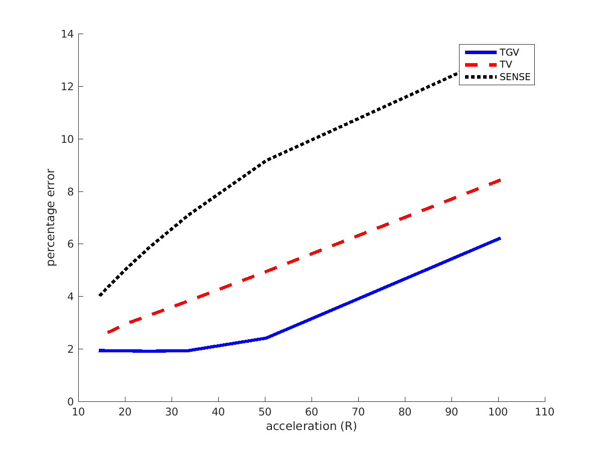
Once the image-space signal is reconstructed, $$$T_1$$$ fitting is done voxel-wise using the approach described in [1].The FS dataset was used as a ground truth to compare the TGV, TV and SENSE results to. The error is measured as, $$$ e^{(RT)} = \sum_{v} |\frac{T_{1}^{(RT)}(v) - T_{1}^{(FS)}( v)}{T_{1}^{(FS)}(v)} | $$$, where the summation is over all voxels in the brain, $$$T_{1}^{(FS)}$$$ and $$$ T_{1}^{(RT)}$$$ are the $$$T_{1}$$$ values of FS and of different reconstruction techniques respectively.
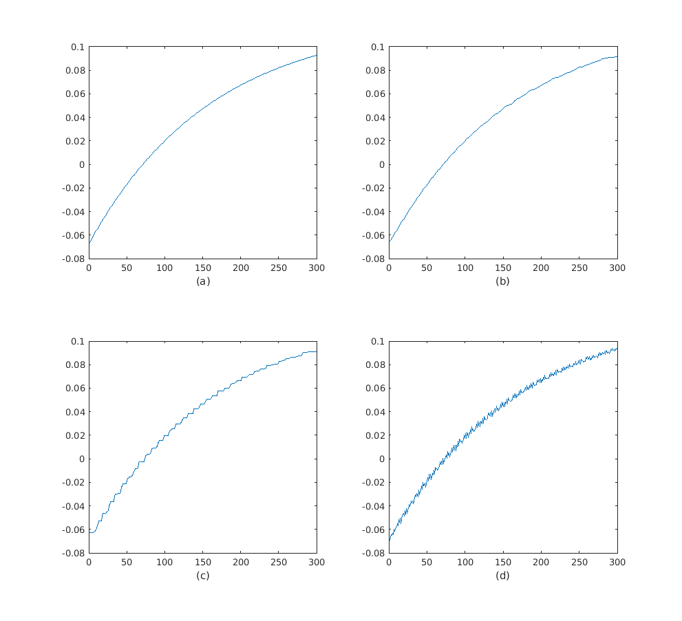
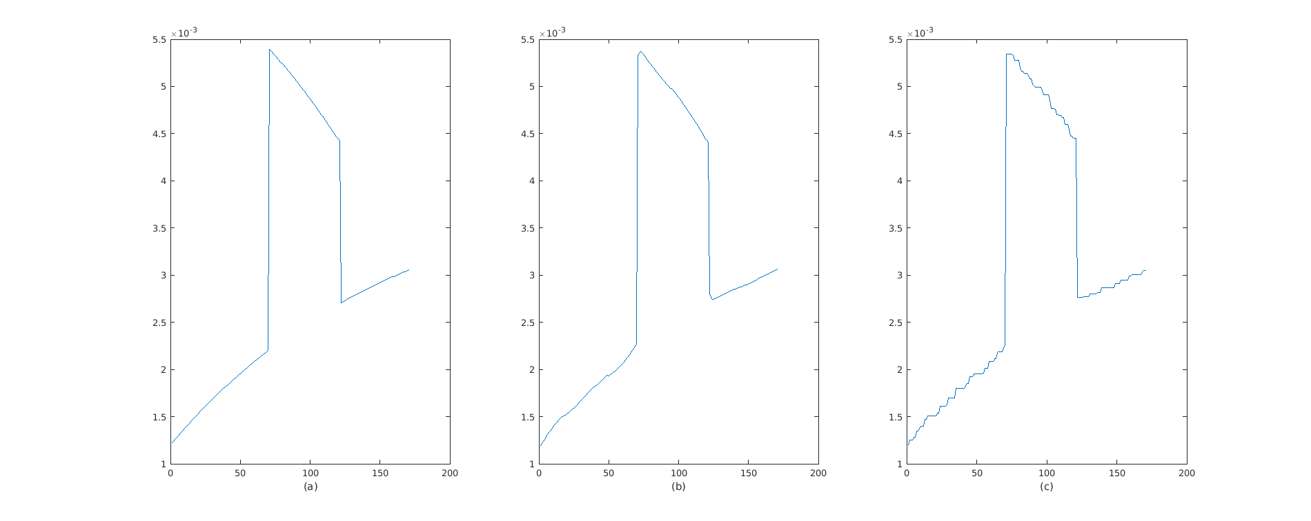
To illustrate the ability of TGV to preserve discontinuities, a synthetic signal whose image-space time course at each voxel has sudden jumps as shown in Figure 5 is used. More details are given in the caption. The procedure discussed earlier for the reconstruction of image-space from k-space is carried out and validation is done visually.
Results
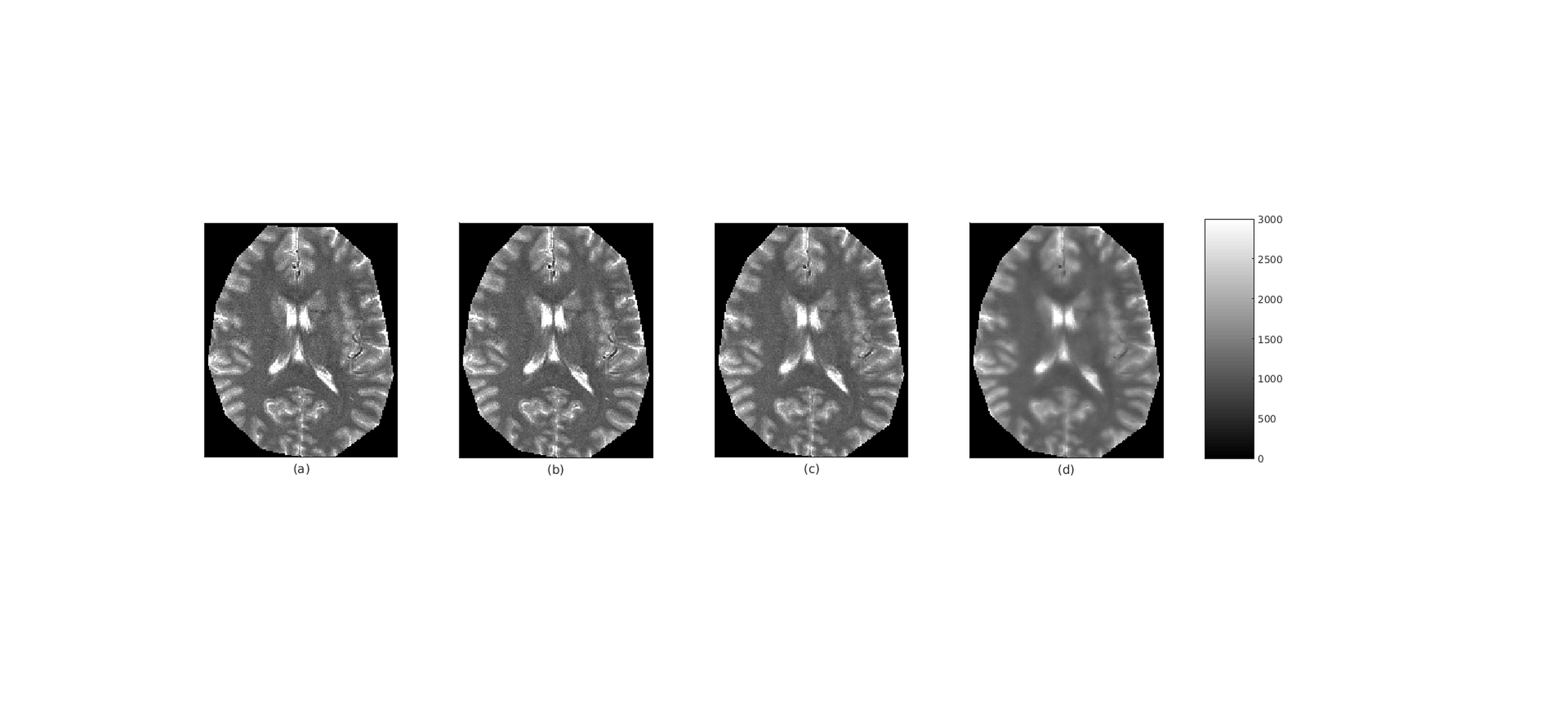
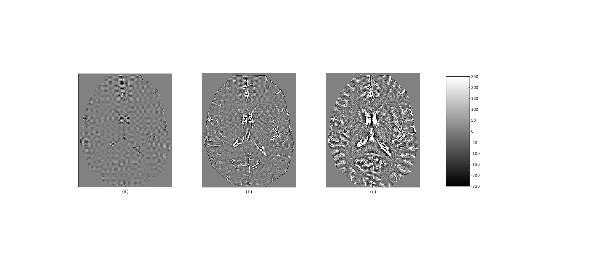
Please refer to the figures and captions for results.Discussion
The fine temporal sampling of MPnRAGE means that the signal at each voxel is slowly varying in time, and this temporal redundancy is exploited by TGV to give a smooth output shown in Figure 4. SENSE gives a relatively small error even at high accelerations because the interleaved radial sampling undersampling artifacts approximate zero-mean additive noise that is generally tolerated well in the $$$T_1$$$ fitting procedure. TGV reduces the variance of this noise producing better $$$T_1$$$ estimates than SENSE. While TV smoothes the signal across time, its output is piecewise constant, which is not the underlying true signal, and hence gives worse $$$T_1$$$ estimates than TGV.TGV outperforms TV for the discontinuous signal of Figure 5 because of reasons given in the description of TGV in the Methods section.
Acknowledgements
This research was made possible with support of National Institutes of Health (NIH) grants HD079119 and HD003352.References
[1] Steven Kecskemeti, Alexey Samsonov, Samuel A. Hurley, Douglas C. Dean, Aaron Field, and Andrew L. Alexander. Mpnrage: A technique to simultaneously acquire hundreds of differently contrasted mprage images with applications to quantitative $$$T_1$$$ mapping. Magnetic Resonance in Medicine, 75(3):1040–1053, 2016.
[2] Florian Knoll, Kristian Bredies, Thomas Pock, and Rudolf Stollberger. Second order total generalized variation (tgv) for mri. Magnetic Resonance in Medicine, 65(2):480–491, 2011.
[3] Klaas P. Pruessmann, et al. "Advances in sensitivity encoding with arbitrary k-space trajectories." Magnetic Resonance in Medicine 46.4 (2001): 638-651.
Figures