3847
Multi-slice extension of iVASO for absolute cerebral blood volume mapping using a 3D GRASE readout1Radiology, University of Washington Medical Center, Seattle, WA, United States, 2Radiology and Radiological Sciences, Vanderbilt University Institute of Imaging Science, Nashville, TN, United States, 3Biomedical Engineering, Vanderbilt University School of Medicine, Nashville, TN, United States, 4Physics and Astronomy, Vanderbilt University School of Medicine, Nashville, TN, United States, 5Radiology, Johns Hopkins University, Baltimore, MD, United States, 6Neurology, Vanderbilt University School of Medicine, Nashville, TN, United States
Synopsis
We present a multi-slice approach to evaluate arterial cerebral blood volume with non-invasive inflow-vascular space occupancy (iVASO) approach using a 3D GRASE readout in conjunction with the iVASO preparation pulses.
PURPOSE
Cerebral blood volume (CBV) is an important physiologic variable relevant to mechanistic BOLD fMRI investigations as well as studies of autoregulation in cerebrovascular disease1-3. CBV is commonly measured using Gadolinium contrast agents and while non-invasive cerebral blood flow measurements have become widely developed, absolute CBV mapping remain comparatively underdeveloped. Recent studies indicate that some Gadolinium is retained by, and may adversely affect neuronal tissue4, thereby stimulating the development of alternative approaches. Inflow vascular space occupancy (iVASO) sequences provide estimates of arterial CBV (aCBV) without exogenous contrast by subtraction of images with and without blood water nulling5-9. Magnetization preparation may consist of a non-selective adiabatic inversion followed by a volume-selective adiabatic inversion for the null image, and two consecutive volume-selective adiabatic inversion pulses for the control image to match magnetization transfer effects. Fundamental limitations of this approach relate to single-slice coverage, draining venous signal from blood water outside the imaging slice, and blood arrival time variations. The purpose of this work was to develop an iVASO protocol that improves spatial coverage using a single-shot 3D GRASE readout and records blood arrival times.METHODS
Experiment: Healthy subjects (n=10; age=25±3years; gender=4F/6M) provided informed, written consent. We performed sequential 3D T1-weighted, single-slice EPI iVASO, and multi-slice iVASO (3D GRASE) acquisitions using body coil transmission and SENSE 32-channel reception (3T; Philips Achieva). Due to uncertainties in blood arrival time, iVASO acquisitions were performed at multiple TIs by adjusting TR and TI to keep the steady-state blood water signal nulled in null acquisitions. Parameters for the single-slice acquisition: matrix = 80×80×12, spatial resolution = 2.75×2.75×5 mm3, flip angle = 90°, TE = 19 ms, TR/TI = 1495/914, 1778/989, 2186/1064, 5000/1191 ms, 30 control/null pairs and an M0 image without iVASO preparation at TR = 10000 ms. The multi-slice imaging parameters were identical except: TE = 22 ms, and 3D GRASE included: k-space profile=low-high, turbo direction=Z, readout duration = 272 ms, SENSE factor = 2.5 (RL) and 2 (AP). Analysis: aCBV was calculated using $$aCBV = \frac{\Delta S}{AM0_{b}C_{b}(\frac{T1b}{\tau})E1E2}$$, where ΔS = difference between control and null images, TI= inversion time, M0b = steady state longitudinal blood magnetization, blood water density Cb =0.87, A = constant related to scaling and scanner gain. $$E1 = 1-e^{\frac{-TR}{T1b}}$$, $$E2 = e^{\frac{-TE}{T2*b}}$$. T1b=1.65s and R2*b = 1/T2*b=16 s-1 are the T1 and R2* of arterial blood respectively, and τ = 1.1s is the blood arrival time. AM0b was calculated using the M0 image6,9. Gray matter (GM) tissue was segmented using the T1 image and GM aCBV values were recorded. The single-slice EPI acquisition was registered to the 3D GRASE image using FLIRT (2D flag). GM aCBV within the registered slice was compared between the two acquisitions, using a paired t-test and with Bland-Altman plots.
RESULTS
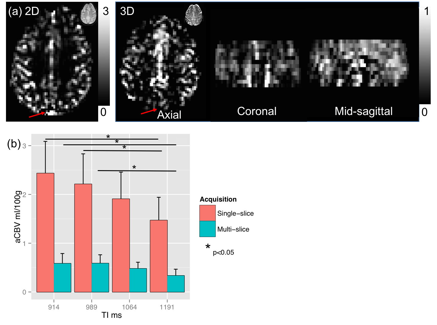
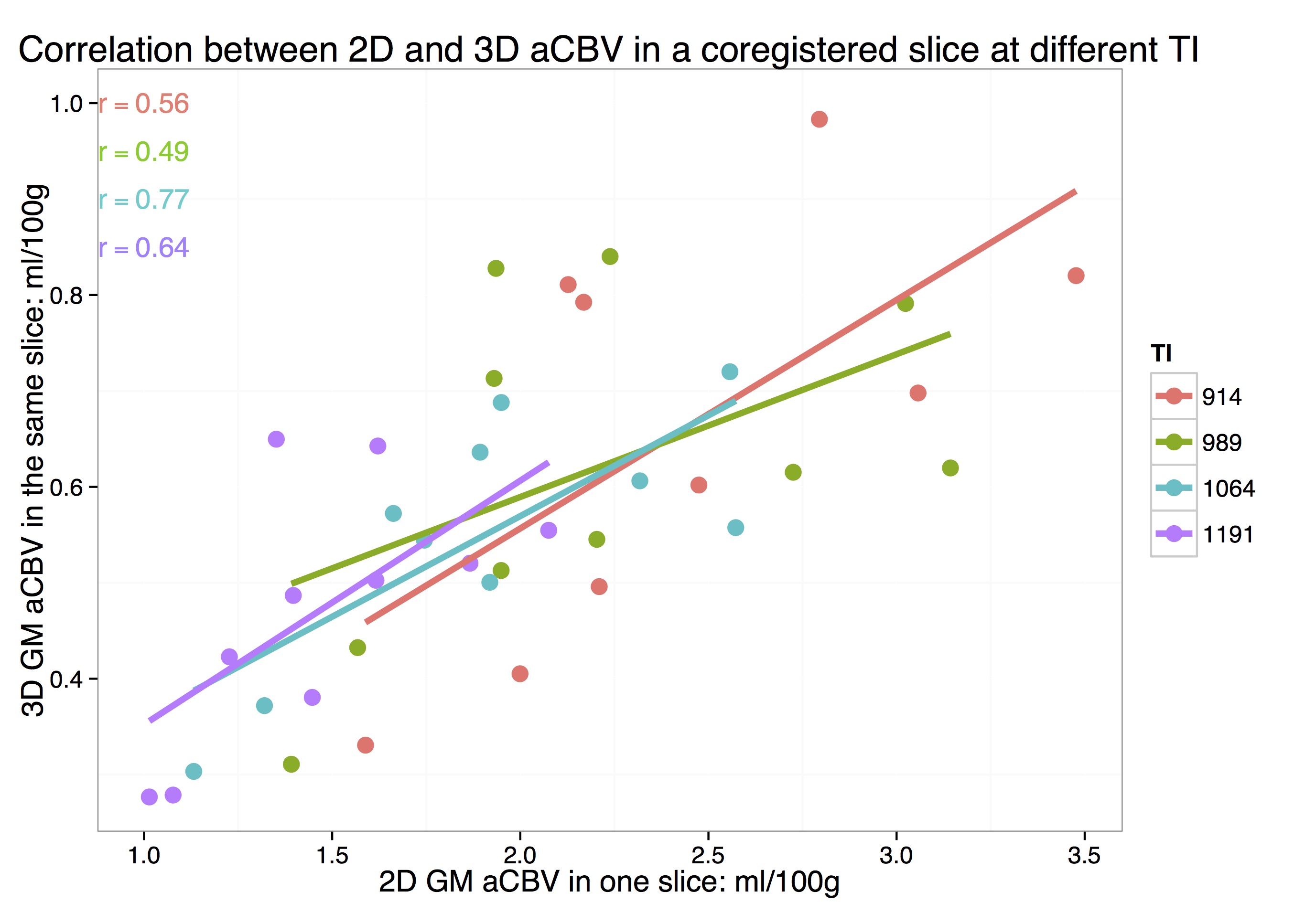
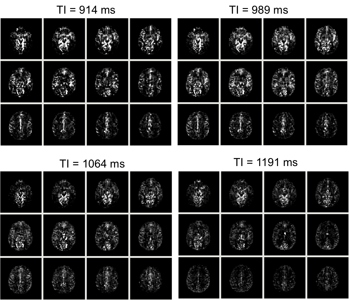
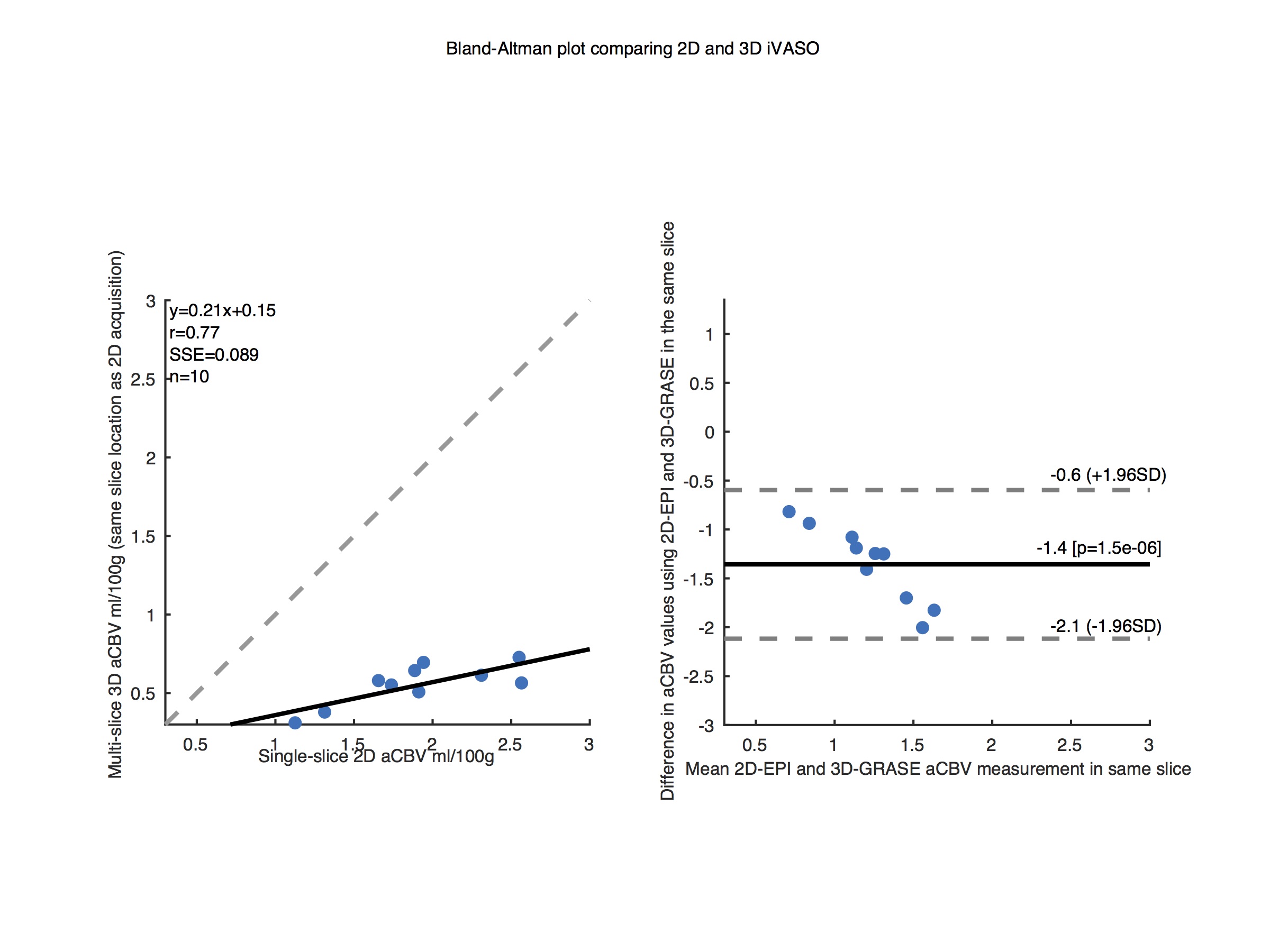
Mean GM aCBV at TI of 914, 989, 1064, and 1191 ms was 2.5±0.6, 2.2±0.6, 1.9±0.5, 1.5±0.3 ml/100g, respectively, with the single-slice iVASO acquisition. aCBV with the multi-slice acquisition was 0.7±0.2, 0.6±0.2, 0.5±0.1, 0.5±0.1 ml/100g, respectively in the same slice. Significant differences (p<0.05) were noted between aCBV values at TI = 1191, and 914 and 989 ms in both acquisitions. aCBV values with 3D GRASE acquisition were consistently significantly lower than with the single-slice readout (Figure 1, p<0.01). Whole-brain GM aCBV values with the 3D acquisition were 0.7±0.1, 0.7±0.2, 0.6±0.1, 0.5±0.1 ml/100g. Figure 2 shows correlations between the single-slice aCBV and aCBV value in the same slice from the multi-slice acquisition at each TR/TI. Figure 3 shows aCBV maps from the multi-slice acquisitions at all TR/TIs. The Bland-Altman plot in Figure 4 shows proportional error i.e., as aCBV value increases, discrepancy between values obtained with the two acquisitions increases.DISCUSSION
We
extended the single-slice iVASO approach to a multi-slice acquisition . τ for
cortical GM is approximately 935±108 ms10, hence cortical GM aCBV is
estimated to be 0.7 ml/100g using this approach. Typically, GM aCBV is 30% of
total CBV ~ 4 ml/100g. We assumed a constant τ for all imaging slices, but τ
can be varied based on arterial geometry and related blood arrival times. The
single-slice acquisition had significant contributions from draining veins in
addition to the pre-capillary arterial vessels. The multi-slice measurements may
be more specific to the pre-capillary network (~30% of the total CBV). This is
evident in Figure 1 where the sagittal sinus appears bright in
the single-slice acquisition but not with the GRASE acquisition. This is also
consistent with the proportional error in the Bland-Altman plot shown in Figure
4.
CONCLUSION
We have improved abilities to measure aCBV using multi-TI iVASO with 3D GRASE.Acknowledgements
No acknowledgement found.References
1. Griffeth VE, Buxton RB. A theoretical framework for estimating cerebral oxygen metabolism changes using the calibrated-BOLD method: modeling the effects of blood volume distribution, hematocrit, oxygen extraction fraction, and tissue signal properties on the BOLD signal. Neuroimage. 2011 Sep 1;58(1):198-212.
2. Donahue MJ, Stevens RD, de Boorder M, Pekar JJ, Hendrikse J, van Zijl PC. Hemodynamic changes after visual stimulation and breath holding provide evidence for an uncoupling of cerebral blood flow and volume from oxygen metabolism. Journal of Cerebral Blood Flow & Metabolism. 2009 Jan 1;29(1):176-85.
3. Blicher JU, Stagg CJ, O'Shea J, Østergaard L, MacIntosh BJ, Johansen-Berg H, Jezzard P, Donahue MJ. Visualization of altered neurovascular coupling in chronic stroke patients using multimodal functional MRI. Journal of Cerebral Blood Flow & Metabolism. 2012 Nov 1;32(11):2044-54.
4. Kanda T, Fukusato T, Matsuda M, Toyoda K, Oba H, Kotoku JI, Haruyama T, Kitajima K, Furui S. Gadolinium-based contrast agent accumulates in the brain even in subjects without severe renal dysfunction: evaluation of autopsy brain specimens with inductively coupled plasma mass spectroscopy. Radiology. 2015 May 5;276(1):228-32.
5. Hua J, Qin Q, Donahue MJ, Zhou J, Pekar JJ, van Zijl P. Inflow-based vascular-space-occupancy (iVASO) MRI. Magnetic resonance in medicine. 2011 Jul 1;66(1):40-56.
6. Rane S, Talati P, Donahue MJ, Heckers S. Inflow-vascular space occupancy (iVASO) reproducibility in the hippocampus and cortex at different blood water nulling times. Magnetic resonance in medicine. 2015 Jul 1.
7. Poser BA, Norris DG. Measurement of activation-related changes in cerebral blood volume: VASO with single-shot HASTE acquisition. Magnetic Resonance Materials in Physics, Biology and Medicine. 2007 Apr 1;20(2):63-7.
8. Huber L, Goense J, Kennerley AJ, Trampel R, Guidi M, Reimer E, Ivanov D, Neef N, Gauthier CJ, Turner R, Möller HE. Cortical lamina-dependent blood volume changes in human brain at 7T. Neuroimage. 2015 Feb 15;107:23-33.Scouten A, Constable RT. VASO-based calculations of CBV change: Accounting for the dynamic CSF volume. Magnetic resonance in medicine. 2008 Feb 1;59(2):308-15.
9. Donahue MJ, Sideso E, MacIntosh BJ, Kennedy J, Handa A, Jezzard P. Absolute arterial cerebral blood volume quantification using inflow vascular-space-occupancy with dynamic subtraction magnetic resonance imaging. Journal of Cerebral Blood Flow & Metabolism. 2010 Jul 1;30(7):1329-42.
10. MacIntosh BJ, Filippini N, Chappell MA, Woolrich MW, Mackay CE, Jezzard P. Assessment of arterial arrival times derived from multiple inversion time pulsed arterial spin labeling MRI. Magnetic Resonance in Medicine. 2010 Mar 1;63(3):641-7.
Figures