3829
An Image Simulation Tool for 3D TSE Including Flow Effects1Siemens Healthcare, Portland, OR, United States, 2Siemens Healthcare, 3Oregon Health & Science University, Portland, OR, United States
Synopsis
A 3D TSE simulation tool designed as both an educational tool as well as a guide for optimizing protocols is described. The pulse sequence protocol user interface triggers integrated Bloch simulations for a user-defined set of tissues based on current protocol settings including the variable flip angle scheme and reordering mode. The tool models tissue T1 & T2 as well as flow effects. We demonstrate applicability to the issue of flow-induced signal loss in CSF and compare simulations to in vivo measurements. The effects of parameter changes that would otherwise require lengthy in vivo comparisons can now be easily explored.
Introduction
Optimization of 3D TSE (i.e. SPACE, VISTA, CUBE) can be a difficult task. Although general guidance is available1, it can be difficult to predict image quality changes given the large number of parameters which have a complicated effect. The results are also heavily dependent on the T1 & T2 relaxation times of the tissue, as well as any motion effects such as blood or CSF flow2. Previous work3 reported a 3D TSE simulation tool which could be used as both an educational tool as well as a guide for optimizing protocols. The current work extends that tool to additionally include flow effects and we demonstrate applicability to the issue of flow-induced signal loss in CSF.Methods
As previously reported3, the simulation software was implemented in C++ directly in the scanner pulse sequence programming environment (IDEA, Siemens). The standard pulse sequence user interface is used to trigger integrated Bloch simulations based on the current protocol settings for a user defined set of tissues. The simulations include a velocity-dependent dephasing term as described by Busse2 of the form Φn = 2πv(nτ) / δx, where Φn is the phase accrued by an isochromat during interval n, v is the velocity of constant motion, τ is defined by convention as half the echo spacing, and δx is the voxel size.
A configuration file defines the relevant properties of the tissue classes to be simulated (T1, T2, PD) as well as the expected average velocity. A template image where each gray level corresponds to one of the tissue classes is Fourier transformed and weighted in k-space according to the signal simulations and the requested phase encoding reordering scheme. The final image is then generated by an inverse Fourier transform. The signal of each tissue throughout the echo train is exported, along with a graphical summary of the reordering scheme. The simulation output is easily visualized by an external viewer program.
Experiments were performed on a Prisma 3T (Siemens) with the following parameters: TE/TR=408/3200ms (T2-weighted), turbo factor=282, sagittal, non-selective excitation, CAIPI acceleration 2x2, (1mm)3 voxels in 2:31. Images were acquired with the standard amount of gradient spoiling along the readout gradient axis, and again with twice the gradient spoiling moment.
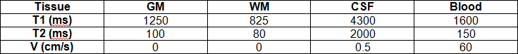
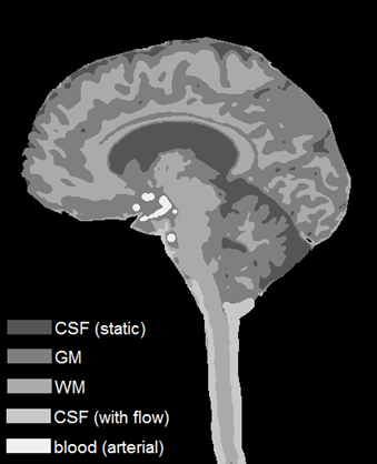
Template images were generated by taking one of the acquired sagittal images and segmenting it into GM/WM/CSF tissue classes. The CSF near the brainstem was segmented into an additional class to include flow effects, and another tissue class was manually drawn to represent the major arteries. A summary of the simulated tissue parameters is shown in Table 1.
The exact protocols as scanned were then simulated using the template image and compared to the in vivo measurements.
Results
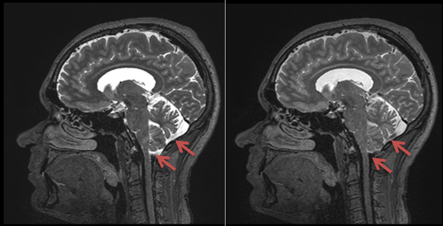
Figure 1 shows a central sagittal image acquired using standard spoiling (left) and double the spoiling (right) along the readout gradient axis (vertical axis in the image). For standard spoiling, CSF signal loss is evident around the spinal cord, and partial CSF signal loss is seen at the base of the cerebellum, as is common with 3D TSE. With double spoiling, more of the CSF in the base of the cerebellum exhibits signal loss.
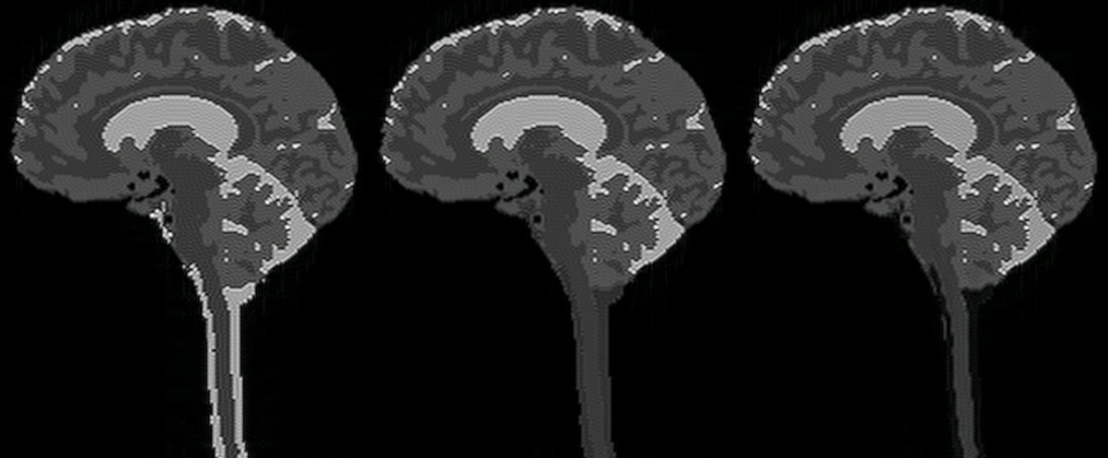
The template image derived from the in vivo image is in Fig. 2. The simulated images in Fig. 3 show the case of no CSF flow for standard spoiling (left), with CSF flow effects for standard spoiling (middle), and with CSF flow effects for double spoiling (right).
Discussion
The reduction of CSF signal with flow and increased spoiling mimics what was seen in vivo. The blood was uniformly dark in all cases due to the much higher velocity, and again the simulations matched what was seen in vivo.
Normally flow-induced dephasing in 3D TSE occurs for motion along the readout axis which is typically the axis of gradient spoiling. Here, it was assumed to dephase for motion along the phase encoding axis (CSF flowing through-plane) to enable simultaneous visualization of phase encoding blurring and flow effects.
A straightforward extension of this tool would be to simulate pulsatile flow. This may be useful in exploring cardiac cycle timing effects on CSF and blood signal and how best to reduce or maximize them.
All allowable protocol-specific RF and gradient timings, variable flip angle optimizations, and reordering schemes are automatically known to the Bloch simulation software via the pulse sequence user interface. The described simulation tool makes it easy to explore the effects of various optimizations that would otherwise require lengthy in vivo comparisons which are prone to limitations such as subject motion.
Acknowledgements
Thanks to William Woodward and Emile Averill of the OHSU Advanced Imaging Research Center for assistance with data acquisition.References
1. Mugler. Optimized Three-Dimensional Fast-Spin-Echo MRI. Journal of Magnetic Resonance Imaging, (2014) 39:745-767.
2. Busse, et al. Effects of Refocusing Flip Angle Modulation and View Ordering in 3D Fast Spin Echo. Magnetic Resonance in Medicine, (2008) 60:640–649.
3. Koerzdoerfer. Simulation of SPACE Imaging. European Society for Magnetic Resonance in Medicine and Biology Book of Abstracts #671, Magn Reson Mater Phy (2015) 28:1.
Figures