3791
Optimisation of Fast Field-Cycling MRI pulse sequences by numerical simulation.1University of Aberdeen, Aberdeen, United Kingdom
Synopsis
Fast Field-Cycling MRI (FFC-MRI) has the ability to access contrast invisible to conventional scanners – that resulting from the dependence of T1 on magnetic field strength. Simulating FFC-MRI sequences by iteratively applying the Bloch equations as the magnetic field strength changes with time was found to give highly accurate predictions of signal intensity at the end of each cycle. This information was used to optimise parameters of the FFC-MRI scans.
Introduction
Fast Field-Cycling MRI (FFC-MRI) is able to access contrast derived from the variation of T1 with magnetic field strength, known as T1-dispersion, which is invisible to conventional MRI.1 This can be seen by either measuring full T1-dispersion data, normally achieved in vivo by using the fast two-point 2-3 or by differences in the signal intensity following fast field-cycling. For either method the choice of evolution time, the time spent at the magnetic field strength of interest, has a strong influence on the results. This is particularly the case if the T1-dispersion curve of the sample contains quadrupole dips, features caused by cross-relaxation of the protons with resonant quadrupolar nuclei such as 14N.4 Such features are present in a number of tissues including muscle, cartilage, and brain.5-7 It is therefore useful to optimise parameters, including evolution time, prior to conducting potentially lengthy scans, in order to maximise sensitivity.Methods
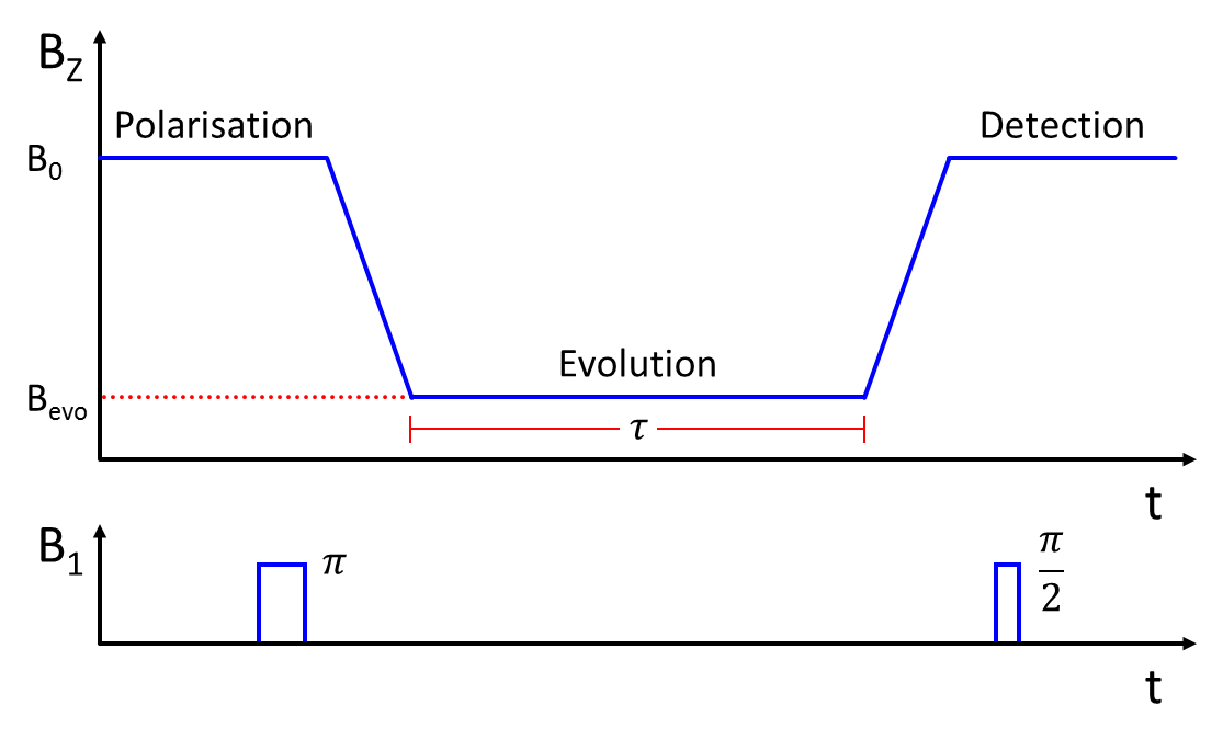
A simulation of a Fast Field-Cycling Inversion Recovery sequence (Fig. 1) was written using MATLAB (The MathWorks Inc., U.S., version 2013a). By mapping a-priori T1-dispersion data onto the known variation in the magnetic field during each experimental cycle, the T1 of the sample was predicted as a function of time during the pulse sequence. The Bloch equations were then used to track the longitudinal magnetisation of the sample throughout the experiment; this was denoted as the ‘signal’ at the point of the 90°-pulse. Time increments of 100 μs were used in the simulation as a compromise between accuracy and computing time. Parameters such as initial polarisation and inversion efficiency were included to closely model the experiment as conducted on a real FFC-MRI scanner. The script was easily adapted to report back any parameter of interest which could then be optimised.
A home-built FFC-MRI scanner1 was used for all scans. The whole-body scanner has a native field, produced by a permanent magnetic, of 59 mT which can be either enhanced or opposed by driving current through a secondary, resistive magnet located within the bore. All elements of the scanner are controlled using a commercial console (MR Solutions Ltd., U.K.) with pulse sequences written or adapted in-house.
Verification and results
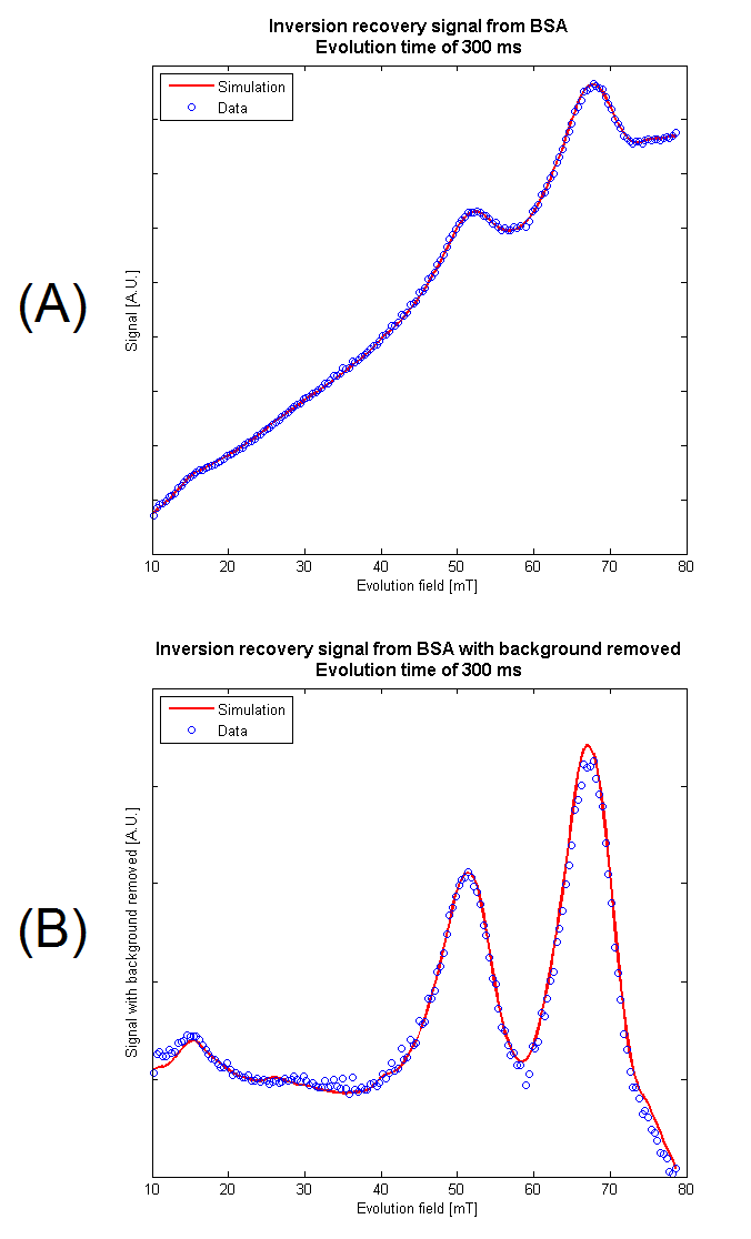
A sample of cross-linked bovine serum albumin (BSA) was chosen for model verification due to the strong quadrupole dips in its dispersion curve. After scaling, the simulation was found to match the data with an R-squared value of >0.995 at a number of evolution times and field strengths (Fig. 2a). By assuming a linear fit, the background signal was removed (Fig. 2b) showing the variation in signal intensity due to the Larmor frequency of the protons becoming equal to a nuclear quadrupole resonance (NQR) frequency of coupled quadrupolar nuclei, allowing cross-relaxation to occur. With an appropriate choice of evolution time, the peak intensities are indicative of the features in the T1-dispersion of the sample.
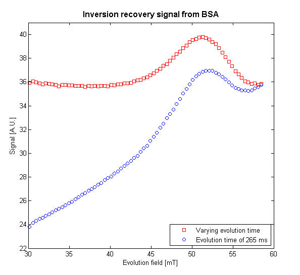
To demonstrate the utility of the simulation, the evolution time was optimised to give the largest difference between the signal and the background for the peak which occurs at 51.5 mT; this was found to be 295 ms. The simulation was then used to output evolution times as a function of evolution field strength such that the background signal would be a constant. This level was set to equal the signal detected with an evolution field of 58.6 mT and an evolution time of 285 ms. From the results shown in Fig. 3, it can be seen that, by normalising the background signal, the peak’s shape is preserved and there is an added benefit of increasing the signal of scans conducted at lower evolution fields, thus improving the signal-to-noise ratio.
Discussion
It has been shown that simulations of FFC-MRI sequences can accurately predict their results. These simulations can be used to optimise experimental parameters for given criteria and, although the results given here were achieved using known T1-dispersion data, it would also be possible to use estimated T1-dispersion behaviour in order to guide the choice of pulse sequence parameters prior to experimentation. Simulation is rapid compared to experimental optimisation and can lead to useful improvements in signal. Furthermore, the simulation is capable of using arbitrary evolution field shapes, allowing for investigation of hypothetical experiments without needing to code the sequence on the MRI console.Conclusion
Simulations of FFC-MRI sequences based on iteratively applying the Bloch equations has proven to be a useful tool in experimental design and although its efficacy depends on accurate T1-dispersion data, it can be used as an initial guide where none is available.Acknowledgements
The author acknowledges funding from the EPSRC through the Centre for Doctoral Training in Integrated Magnetic Resonance.References
1. Lurie, D.J. et al. Fast field-cycling magnetic resonance imaging. Comptes Rendus Phys. 2010;11:136-148.
2. Edelstein, W.A. et al. Spin warp NMR imaging and applications to human whole-body imaging. Phys. Med. Biol. 1980;25:751-756.
3. Broche, L.M. et al. Rapid multi-field T1 estimation algorithm for Fast Field-Cycling MRI. J. Magn. Reson. 2014;238:44-51.
4. Edmonds D.T. Nuclear quadrupole double resonance. Phys.Rep. 1977;29(4):233-290.
5. Winter, F. and Kimmich, R. NMR field-cycling relaxation spectroscopy of bovine serum albumin, muscle tissue, micrococcus luteus and yeast. Biochim. Biophys. Acta. 1982;719:292-298.
6. Koenig, S.H. and Brown, R.D. Field-cycling relaxometry of protein solutions and tissue: Implications for MRI. Prog. Nucl. Mag. Res. Sp. 1990;22:487-567.
7. Broche, L.M., Ashcroft, G.P. and Lurie, D.J. Detection of osteoarthritis in knee and hip joints by Fast Field-Cycling NMR. Magn. Reson. Med. 2012;68:358-362.
Figures