Introduction

The Superior Colliculus is located in the midbrain and is a paired layered structure that regulates eye and head movements and is involved in multisensory control. It is divided in 7 alternating fibrous and cellular layers and our goal is to find imaging methods with improved contrast in the midbrain, ideally capable of separating the SC layers in- vivo. In particular the superficial layer is known to be composed of myelinated axons receiving inputs mostly from the retina. In this study the visibility of midbrain structures with different MR contrasts in vivo was assessed. In particular we investigated the SC boundaries and its layering structure in-vivo at 9.4T and validated with ex-vivo measurements at 9.4T, 14T and polarized light imaging (PLI).

Methods

For the in-vivo measurements 11 subjects were measured at 9.4T (Siemens, Erlangen,Germany). For each participant three different sequences were used: acquisition-weighted (AW) [1] (nominal resolution of 0.175x0.132x0.6mm; TE=18ms), multi-echo (ME) 3D GRE (0.4mm isotropic resolution, TE=6:6:36ms), and whole brain MP2RAGE (0.8 isotropic resolution). The AW images were k-space filtered with a Hanning function in the phase encoding dimension [2] in order to increase the SNR. Quantitative MR analysis was performed: R1 maps were calculated from the MP2RAGE sequence after B1 correction[3]; R2* maps were calculated from the ME images using the NumART method [4]; and quantitative susceptibility maps (QSM) were calculated using the raw data obtained with the AW sequence. For calculating QSM the phase images were unwrapped and the background field was removed using the RESHARP algorithm[5], the inverse problem was solved using the least squares approach [6]. In order to highlight the SC structure that is common across subjects, the images were registered to MNI space using DARTEL in their original resolution, implemented in SPM12. VOIs of the SC, red nucleus (RN), aqueductal gray (AG) were drawn using the R2* maps, in individual space for each subject and in MNI space. All the images and VOIs were translated to the AW space for contrast to noise ratio (CNR) calculation. The CNR between the SC and a WM VOI was calculated. The post-mortem brainstem sample was fixed in formalin (4%), measured in the 9.4T using the in-vivo protocol, and then cut to fit the 14T volume coil. At 14T, 3D GRE (50μm isotropic resolution), multi gradient echo (MGE) (100 μm isotropic resolution and DTI GRE (6dir, b=10000, 300μm isotropic resolution) were acquired. After the 14T measurement the sample was sliced and PLI images were acquired.

Results

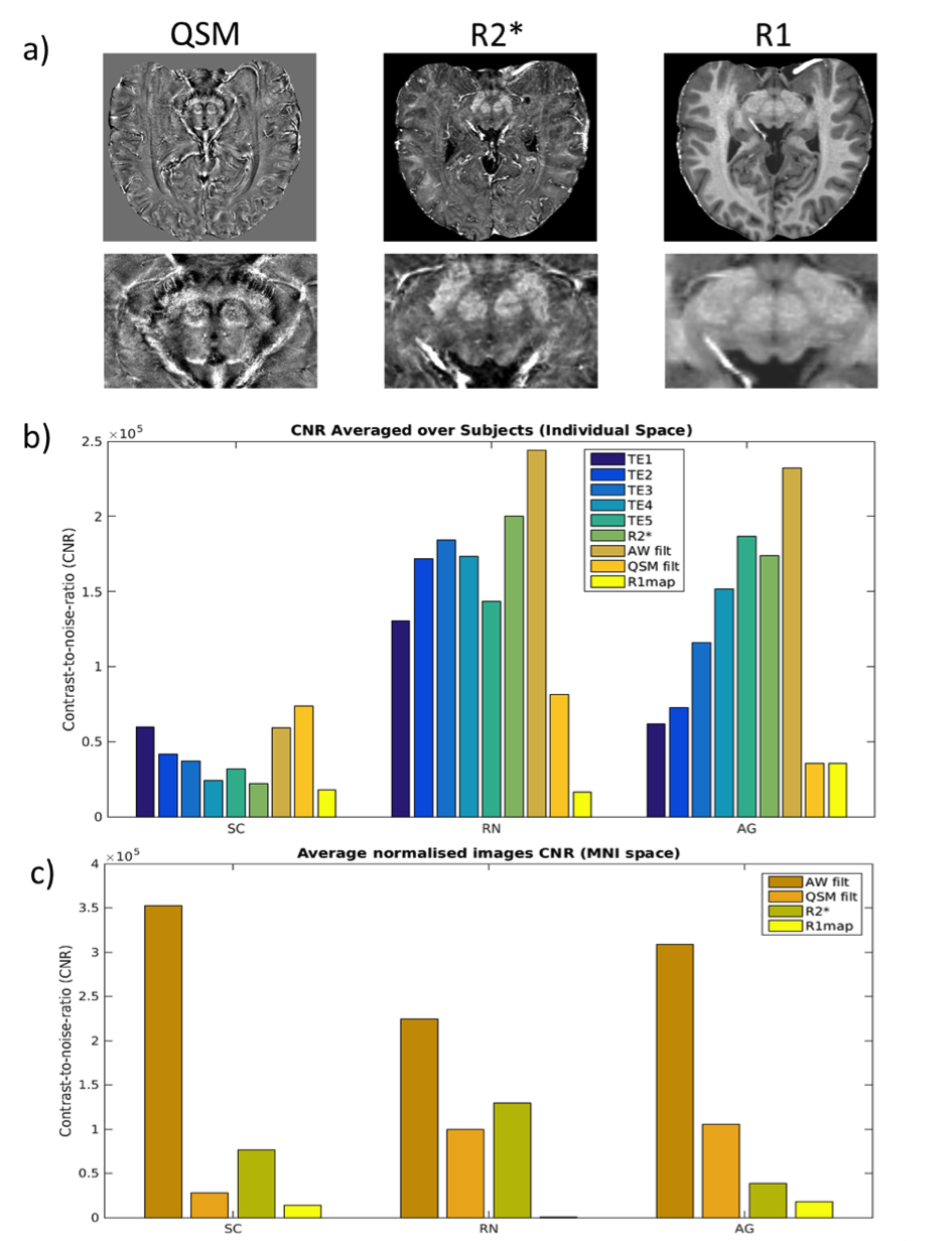
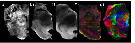
Fig.1a) shows quantitative MR images obtained for one subject (QSM, R2* and R1 maps), and Fig.1b) and c) show the CNR results obtained in-vivo in individual space averaged across subjects, and in MNI space respectively. In individual space (Fig.1b)), we obtained enhanced contrast with the quantitative R2* map for the RN and AG in comparison with the individual echoes. However, the contrast was not improved in the SC. QSM maps increased substantially the CNR in the SC but not in the RN and AG comparatively with the amplitude images from the AW sequence. For all the structures the R1 map gave the lowest CNR values. For the CNR obtained from the averaged normalized MNI images (Fig.1c)), we obtained highest CNR with the AW magnitude images for all the structures. The GRE ex-vivo images were comparable to the in-vivo images. The first eigenvector of the DTI images show the superficial layer in accordance to its anatomy and also a layering structure in the middle part of the SC, which may represent one of the intermediate layers of the SC. This layering structure was also obtained in the PLI images. To note that the color code of the DTI (3D) and the PLI (2D) are distinct and the fibre orientation cannot be directly compared between the two modalities (Fig.2).

Discussion

Quantitative R2* mapping and QSM imaging provided higher CNR in deep brain structures. In particular an increase in CNR was observed in QSM maps in the SC. QSM maps not only gave more insight about the SC boundaries but also about its layering structure showing an increase in susceptibility in the superficial zone of the SC which is likely due to the presence of myelinated neuronal fibre bundles detected by DTI and PLI in the superficial layer.

Conclusion

This study emphasizes the potential of UHF MRI for measuring deep-brain structures. The use of 9.4T in-vivo and the comparison of this data with ex-vivo samples may enable us to create more robust and accurate atlases of the SC and possibly reveal the layering pattern of the SC.

Acknowledgements

We gratefully acknowledge funding by the Max Planck Society, and the ministry of Science, Research andthe Arts of Baden-Württemberg (Az: 32-771-8-1504.12/1/1, to GH). WThis work was supported by the Carl Zeiss foundation awarded to JL.