3684
Comparison of Quantitative Susceptibility Mapping algorithms based on numerical and in vivo 3T data1Radiology, Leiden University Medical Center, Leiden, Netherlands, 2C.J. Gorter Center for High Field MRI Research, Leiden University Medical Center, Leiden, Netherlands
Synopsis
This study compares the currently publically available algorithms for quantitative susceptibility mapping, including different phase unwrapping, background field removal and dipole inversion methods. Numerical and human in vivo brain MRI data are used for a qualitative and quantitative assessment of the various methods. In 3T in vivo MRI data, phase unwrapping with combined spatial and temporal fitting and background field removal using V-SHARP results in the least artifacts. MEDI and iLSQR are currently the most accurate dipole inversion algorithms, with a significantly shorter processing time for the iLSQR method.
Purpose
Quantitative susceptibility mapping (QSM) provides a sensitive and linear measure for tissue susceptibility on magnetic resonance imaging (MRI) that is relatively independent of orientation.1 Processing stages in QSM include multiple phase unwrapping, background field removal and dipole inversion algorithms and have been implemented in several QSM packages. Lacking is a systematic comparison of these methods. The aim of this study is to perform a comparative evaluation of available QSM algorithms on numerical and in vivo MRI data.Methods
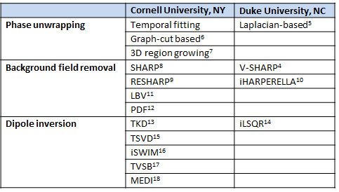
A literature search was performed to select and obtain MATLAB-based algorithms for MRI phase unwrapping, background field removal and dipole inversion (Table 1). The following data sets were acquired from Cornell University, NY for comparing different algorithms:
1. A multi‐echo gradient echo brain MRI from a healthy subject acquired on a Siemens 3T system (8 echoes; TE = 3.6~45 ms; TR = 55 ms; voxel size = 0.9375x0.9375x2 mm3; matrix size = 256x256x642)
2. A numerical brain with a known susceptibility distribution
3. A ground truth data set comprised a QSM map generated by calculation of susceptibility through multiple orientation sampling (COSMOS)2 from five different orientations, based on multi‐echo gradient echo MRI scans from a healthy subject (3T GE system; 10 echoes; TE = 5~50 ms; TR = 55 ms; reconstructed voxel size 0.9375x0.9375x1 mm3; matrix size = 240×240×146). Single orientation data was processed with homogeneity-enabled incremental dipole inversion (HEIDI)3 and compressed sensing compensated (CSC)4 dipole inversion by the providing institute, as these MATLAB codes were not publicly available.
QSM maps from the numerical data and in vivo data were compared to the known susceptibility distribution and COSMOS data respectively using linear regression.
Results
Phase unwrapping
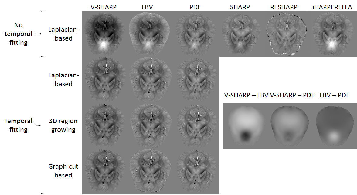
After temporal fitting of the multi-echo data, all phase unwrapping algorithms performed similar on in vivo data. Based on qualitative visual assessment, contrast in tissue phase maps was more dependent on the background field removal method when temporal fitting was not performed (Figure 1).
Background field removal
After Laplacian-based phase unwrapping, SHARP and RESHARP algorithms resulted in discarded voxels at the edges. Susceptibility values in the basal ganglia were underestimated after RESHARP compared to other background field removal methods. Tissue phase maps after Laplacian‐based phase unwrapping combined with iHARPERELLA, LBV or PDF, but not V-SHARP, showed hyperintense regions around the air‐tissue interface of the sinuses, indicating a residual background effect. PDF also resulted in errors at the tissue edges (Figure 1).
Dipole inversion
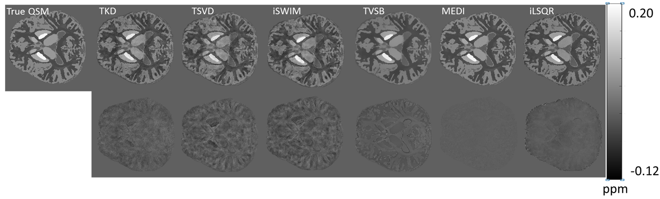
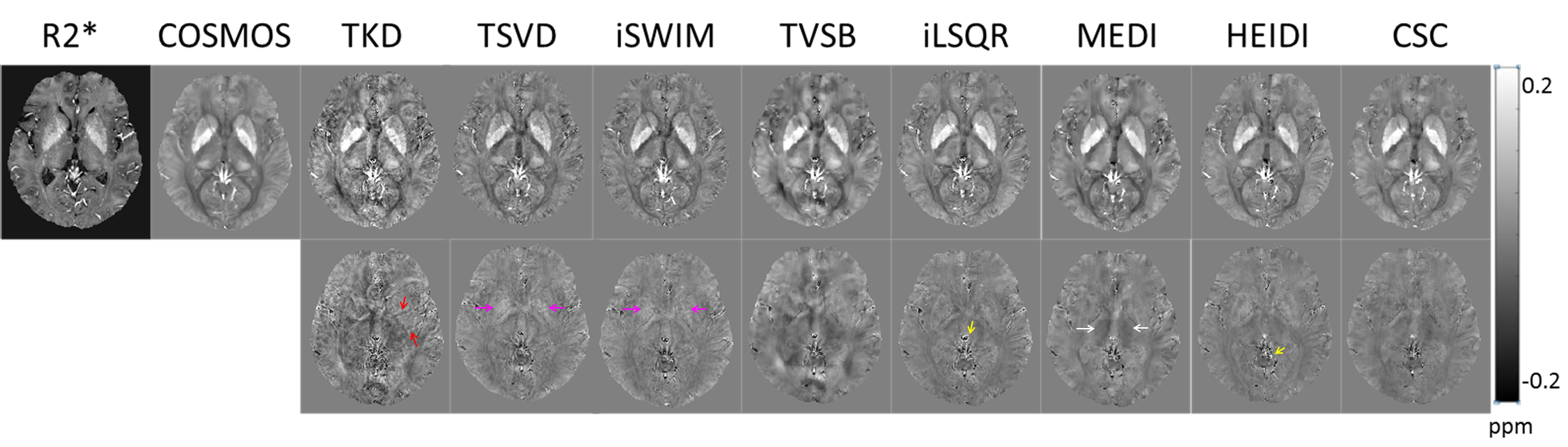
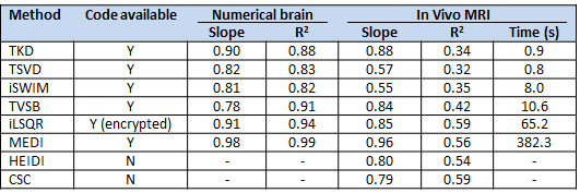
Processing of numerical brain data using different dipole inversion methods showed the best approximation of the true susceptibility values by MEDI with the regularization parameter λ = 3000 (R2 = 0.99), followed by iLSQR (R2 = 0.94) and TVSB (R2 = 0.91) (Figure 2, Table 2). In the in vivo data, Bayesian methods (TVSB, CSC, iLSQR, MEDI and HEIDI) provided QSM maps with determination coefficient closer to 1 than non‐Bayesian algorithms. TKD insufficiently suppressed streaking artifacts, whereas TSVD and iSWIM underestimated susceptibility values in the basal ganglia. TVSB showed overregularization, seen as a cloudy appearance in the difference map, whereas iLSQR, MEDI and HEIDI visually resulted in the most anatomical detail, especially in cortical regions. HEIDI and iLSQR methods yielded more artifacts around veins than other Bayesian methods. MEDI overestimated susceptibility values in the midbrain (Figure 3). Processing time was significantly longer in the Bayesian methods, the MEDI algorithm requires about six times as much processing time as iLSQR dipole inversion (Table 2).
Discussion
Phase unwrapping and background field removal are essential steps for obtaining valid and robust QSM results. Results from V‐SHARP were relatively independent from the phase unwrapping method used, whereas results from other methods were highly influenced by temporal fitting. For dipole inversion, MEDI and iLSQR generated the most accurate results in numerical data and in vivo data, but the regression value compared to COSMOS was only moderate for all dipole inversion methods. This may be due to inaccurate susceptibility estimation in white matter with single orientation acquisitions due to tissue anisotropy.Conclusion
In 3T in vivo MRI data, phase unwrapping with combined spatial and temporal fitting and background field removal using V-SHARP result in the least artifacts. MEDI and iLSQR are currently the most accurate dipole inversion algorithms, with a significantly shorter processing time for the iLSQR method.Acknowledgements
This work was financially supported by a grant from the European Union 7th Framework Program: BrainPath (PIAPP-GA-2013–612360).References
1. Haacke EM, Liu S, Buch S, Zheng W, Wu D, Ye Y. Quantitative susceptibility mapping: current status and future directions. Magn Reson Imaging 2015;33(1):1-25.
2. Liu T, Spincemaille P, de Rochefort L, Kressler B, Wang Y. Calculation of susceptibility through multiple orientation sampling (COSMOS): a method for conditioning the inverse problem from measured magnetic field map to susceptibility source image in MRI. Magn Reson Med 2009;61(1):196-204.
3. Schweser F, Sommer K, Deistung A, Reichenbach JR. Quantitative susceptibility mapping for investigating subtle susceptibility variations in the human brain. Neuroimage 2012;62(3):2083-2100.
4. Wu B, Li W, Guidon A, Liu C. Whole brain susceptibility mapping using compressed sensing. Magn Reson Med 2012;67(1):137-147.
5. Li W, Wu B, Liu C. Quantitative susceptibility mapping of human brain reflects spatial variation in tissue composition. Neuroimage. 2011;55:1645–1656.
6. Bioucas-Dias JM1, Valadão G. Phase unwrapping via graph cuts. IEEE Trans Image Process. 2007;16(3):698-709.
7. Abdul-Rahman H, Gdeisat M, Burton D, Lalor M. Fast three-dimensional phase-unwrapping algorithm based on sorting by reliability following a non-continuous path. Intl Soc Opt Photonics. 2005:32–40.
8. Schweser F, Deistung A, Lehr BW, Reichenbach JR. Quantitative imaging of intrinsic magnetic tissue properties using MRI signal phase: An approach to in vivo brain iron metabolism? Neuroimage. 2011;54(4):2789–2807.
9. Sun H, Wilman AH. Background field removal using spherical mean value filtering and Tikhonov regularization. Magn Reson Med 2014;71(3):1151-1157.
10. Li W, Avram AV, Wu B, Xiao X, Liu C. Integrated Laplacian-based phase unwrapping and background phase removal for quantitative susceptibility mapping. NMR Biomed 2014;27(2):219-227.
11. Zhou D, Liu T, Spincemaille P, Wang Y. Background field removal by solving the Laplacian boundary value problem. NMR Biomed 2014;27(3):312-319.
12. Liu T, Khalidov I, de Rochefort L, Spincemaille P, Liu J, Tsiouris AJ, Wang Y. A novel background field removal method for MRI using projection onto dipole fields (PDF) NMR Biomed. 2011;24(9):1129–1136.
13. Shmueli K, de Zwart JA, van Gelderen P, Li TQ, Dodd SJ, Duyn JH. Magnetic susceptibility mapping of brain tissue in vivo using MRI phase data. Magn Reson Med 2009;62(6):1510-1522.
14. Li W, Wang N, Yu F, Han H, Cao W, Romero R, Tantiwongkosi B, Duong TQ, Liu C. A method for estimating and removing streaking artifacts in quantitative susceptibility mapping. Neuroimage 2015;108:111-122.
15. Wharton S, Schäfer A, Bowtell R. Susceptibility mapping in the human brain using threshold-based k-space division. Magn Reson Med 2010;63(5):1292-1304.
16. Tang J, Liu S, Neelavalli J, Cheng YC, Buch S, Haacke EM. Improving susceptibility mapping using a threshold-based K-space/image domain iterative reconstruction approach. Magn Reson Med 2013;69(5):1396-1407.
17. Bilgic B, Fan AP, Polimeni JR, Cauley SF, Bianciardi M, Adalsteinsson E, Wald LL, Setsompop K. Fast quantitative susceptibility mapping with L1-regularization and automatic parameter selection. Magn Reson Med 2014;72(5):1444-1459.
18. Liu T, Liu J, de Rochefort L, Spincemaille P, Khalidov I, Ledoux JR, Wang Y. Morphology enabled dipole inversion (MEDI) from a single-angle acquisition: comparison with COSMOS in human brain imaging. Magn Reson Med 2011;66(3):777-783.
Figures