3679
Evaluation of air/bone segmentation using susceptibility-based imaging methods1Medical Physics and Biomedical Engineering, University College London, London, United Kingdom, 2Leonard Wolfson Experimental Neurology Centre, University College London, Institute of Neurology, United Kingdom, 3Institute of Nuclear Medicine, UCLH-NHS Foundation Trust, United Kingdom
Synopsis
Due to the difference in magnetic susceptibility of air, teeth and bone, magnetic susceptibility mapping has the potential to enable segmentation of these regions despite the absence of direct MRI signal. Several methods have been described which attempt to calculate the magnetic susceptibility within air and bone. Two datasets are used to test the ability of these methods to distinguish between air and bone. The performance of all methods varied between datasets and depended strongly on the parameters selected. None of the methods performed consistently better across groups, but all showed potential to improve air/bone segmentation using susceptibility mapping.
Introduction
The ability to distinguish air and bone in MRI is desirable in many applications such as attenuation correction for PET-MRI. However, both air and bone are invisible using conventional MRI sequences. As air and bone lie at opposite ends of the magnetic susceptibility (𝜒) spectrum within the human body1 we use the 𝜒 of air and bone to differentiate regions containing air, bone and soft tissue. Due to the absence of phase signal in air and bone, the non-local phase in the surrounding soft tissue is the only available information about the 𝜒 in these “missing phase regions” (MPRs). Here we used four recent methods for calculating the 𝜒 in MPRs and compare the results of segmenting the resulting 𝜒 distributions into air, soft tissue and bone.Methods
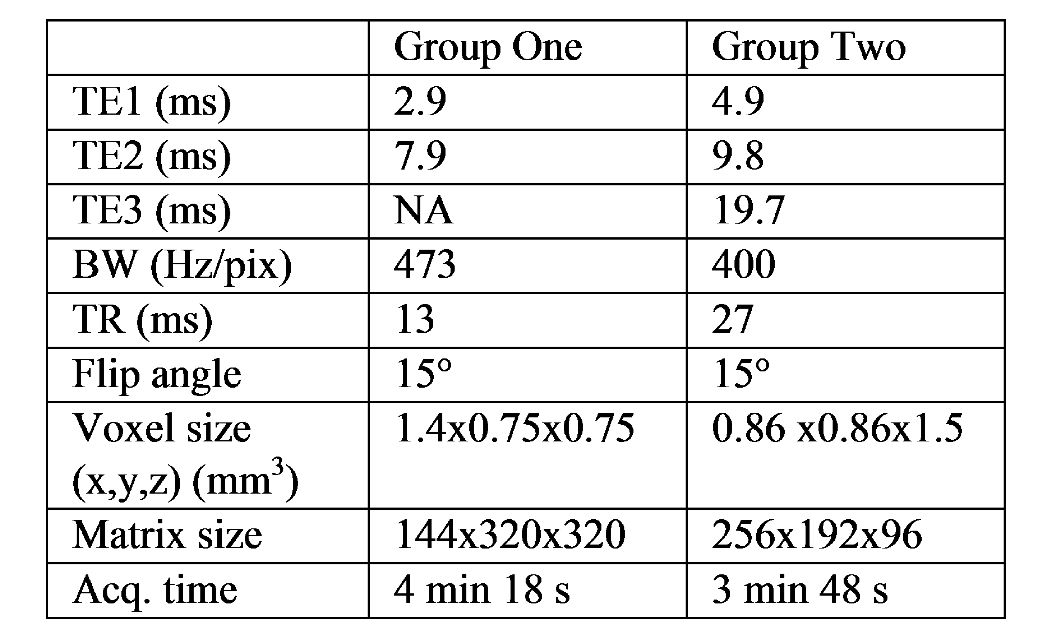
Data were acquired in three healthy volunteers (group one; mean age 27) and 9 subjects from an ongoing PET-MRI study of aging (group two; all aged 69). All images were acquired on a 3T Siemens Biograph mMR system using a 16-channel head and neck coil. The 3D GRE sequence parameters are shown in figure 1. A threshold was applied to TE1 magnitude images to produce a tissue mask which excluded MPRs within the head (i.e. air, bone and teeth). Phase images were unwrapped using PRELUDE2. Large-scale phase variations were removed by quadratic fitting of the TE1 phase. No further background field removal was performed in order to preserve the phase variations resulting from MPRs. Four methods were used to produce susceptibility maps within MPRs: 1. TKD (results shown for 𝛿=0.1)3, with the phase in the low signal regions set to zero, 2. an iterative phase replacement (IPR) method described by Buch et. al.4,5, 3. PDFD: The dipole distribution from PDF6 was used as an approximation of the 𝜒 in MPRs and 4. TFT (Total field inversion with Tikhonov regularisation): based on the principle of preserving all background fields7. Tikhonov regularisation with weighting matrix W was used to calculate 𝜒 in both MPRs and tissue. W is the inverse of the noise standard deviation8 for group two. However, as group one had only two echoes, W was set to equal the tissue mask. The following equation was solved using conjugate gradients $$$\chi^{*}=argmin\frac{1}{2}||\mathrm{{\textstyle W}}\left(\triangle\mathrm{B}-\mathrm{d}\otimes\chi\right)||_{2}^{2}+\alpha||\mathrm{W}\chi||_{2}^{2}$$$ where ΔB is the local field offset, d is the unit dipole field and $$$\alpha=0.05$$$ is the regularisation parameter.
A threshold-based segmentation method9 was applied to the 𝜒 map within the air and bone and the resulting segmentations were compared to a pseudo-CT10 which was also thresholded into the same three tissue classes (i.e. air, bone and soft tissue).
Results
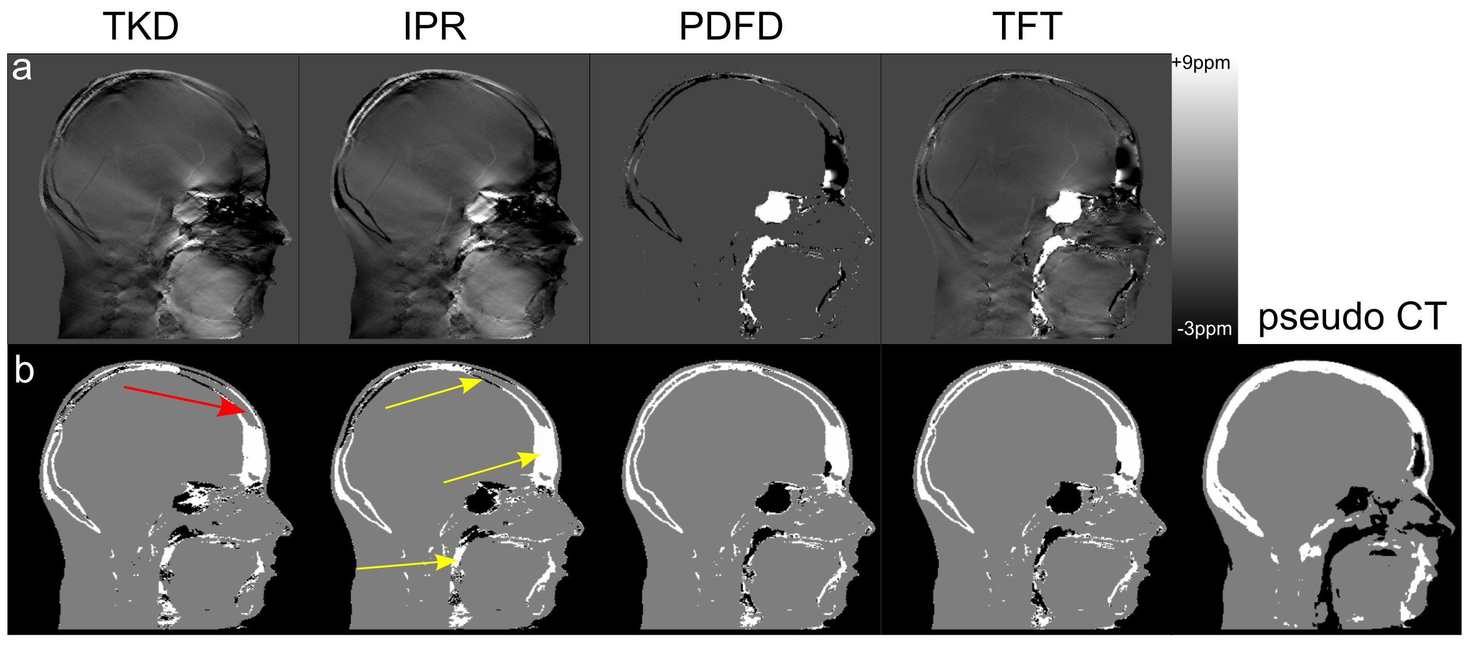
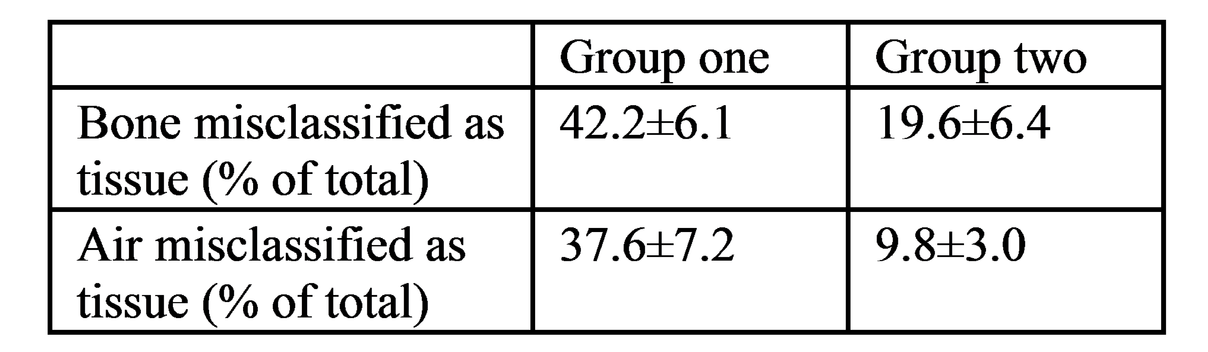
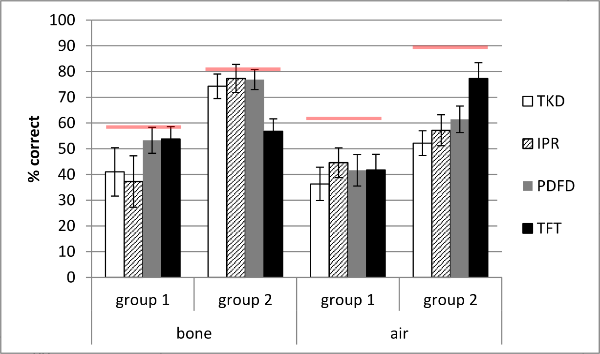
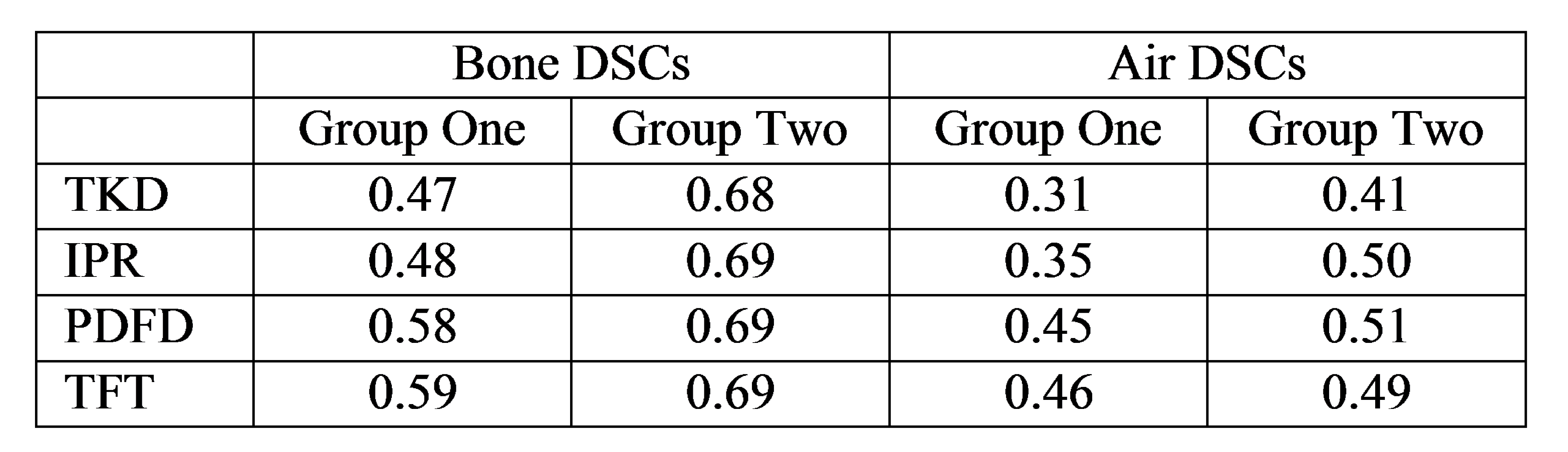
Figure 2 shows tissue class images and 𝜒 maps from a representative subject from group 1. The skull is noticeably thinner in the MRI 𝜒 maps than in the pseudo-CT image due to the initial masking classifying the diploë (red arrow fig 2b) incorrectly as soft tissue. Figure 3 shows the percentages of air and bone misclassified as tissue (using the thresholded pseudo-CT as a gold-standard). Group 1 has much larger misclassifications, probably due to the short TE1, meaning that trabecular bone with T2* longer than cortical bone had non-zero MRI signal and the fact that the larger field of view included the pharynx where much of the air was misclassified as tissue. Figure 4 shows the percentage of correctly segmented air and bone for both groups. Figure 5 shows Dice Similarity Coefficients.Discussion and Conclusion
None of the methods performed consistently better across groups, although IPR and PDFD generally yielded more accurate segmentations than TKD alone as is evident from their DSCs. TFT performed inconsistently across the groups. The initial masking placed a limit on the success of 𝜒-based segmentation as any air and bone included in the tissue mask was misclassified as soft tissue regardless of its 𝜒. Common areas where segmentation failed are the skull, pharynx and sinuses close to the edge of the head (yellow arrows fig 2b), suggesting that both the lack of sufficient surrounding phase information and the orientation relative to B0 have an effect. The relative success of the four methods depended strongly on the initial phase masking, the 𝜒 mapping parameters and the acquisition protocol. Future work will involve validating the segmentations against real CT images in patients having both PET-MRI, including the MRI UTE images currently used for attenuation correction, and CT scans. In order to maintain tissue contrast in addition to contrast between air and bone, TFI with preconditioning will be investigated as in [7].Acknowledgements
No acknowledgement found.References
[1] Schenck "The role of magnetic susceptibility in magnetic resonance imaging: MRI magnetic compatibility of the first and second kinds." Medical physics 23(6) (1996)
[2] Jenkinson, "Fast, automated, N-dimensional phase-unwrapping algorithm", Magn Reson Med 49(1) (2003)
[3] Shmueli et al. "Magnetic susceptibility mapping of brain tissue in vivo using MRI phase data.", Magn Reson Med 62(6) (2009)
[4] Buch et al. "Susceptibility mapping of air, bone, and calcium in the head.", Magn Reson Med 73(6) (2015)
[5] Dixon et al. "Evaluation of an iterative phase replacement method for susceptibility mapping in regions with no MRI signal" Proc. Intl. Soc. Mag. Reson. Med. 24 (2016)
[6] Liu et al. "A novel background field removal method for MRI using projection onto dipole fields (PDF)", NMR Biomed 24(9) (2011)
[7] Liu et al. "Preconditioned Total Field Inversion ( TFI ) method for Quantitative Susceptibility Mapping", Magn Reson Med (2016)
[8] Liu et al. "Nonlinear formulation of the magnetic field to source relationship for robust quantitative susceptibility mapping." MRM 69(2) (2013)
[9] Otsu "A threshold selection method from gray-level histograms", Automatica 11 (1975)
[10] Burgos et al. "Attenuation correction synthesis for hybrid PET-MR scanners : Application to brain studies", IEEE Trans. Med. Imaging 33(12) (2014)
Figures