3677
Resolution and Coverage for Accurate Susceptibility Maps: Comparing Brain Images with Simulations1Department of Medical Physics and Biomedical Engineering, University College London, London, United Kingdom, 2Centre for Medical Imaging, University College London, London, United Kingdom
Synopsis
Magnetic Susceptibility Mapping is moving closer to clinical application. To reduce scan time, clinical images are often acquired with reduced resolution and coverage in the through-slice dimension. The effect of these factors has been studied using only balloon phantoms and downsampled brain images. Here, we used MR images acquired at low resolution or low coverage and compared these with images simulated in volunteers and a realistic numerical phantom. Simulated susceptibility maps were very similar to maps from acquired images. Our results show that low resolution and very low coverage both lead to loss of contrast and errors in susceptibility maps.
Introduction
Magnetic Susceptibility Mapping (SM) is a recently developed MRI technique with emerging clinical applications$$$^{1-2}$$$. Clinical images are often acquired with large slice thickness and reduced coverage in the through-slice dimension$$$^{3-5}$$$ to shorten scans and increase patient comfort and throughput. Recently, the effect of these factors on SM has been studied using a balloon phantom$$$^{6}$$$ and downsampled brain images$$$^{7-10}$$$. Here, we used MR images acquired at low resolution or low coverage and compared these with images simulated in volunteers and an anthropomorphic Zubal head-and-neck, numerical phantom$$$^{11}$$$.Methods
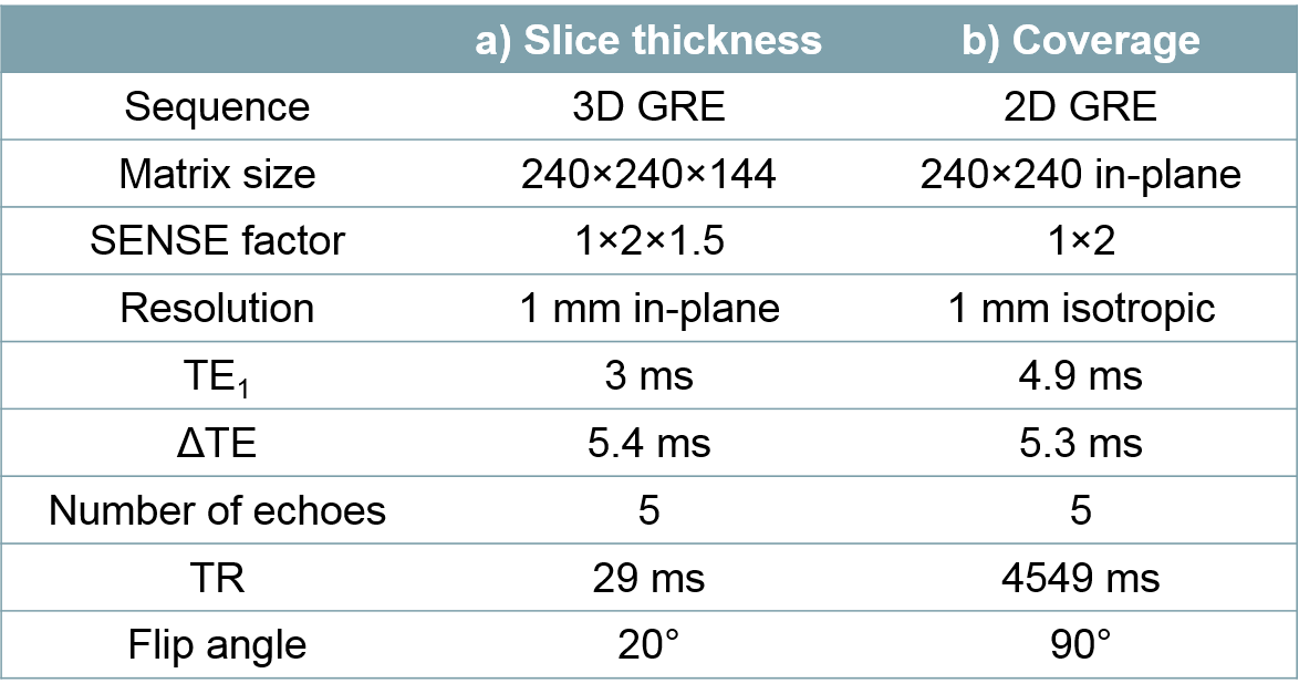
Brain images were acquired in four healthy volunteers at 3-Tesla (Philips, Achieva) using a 3D GRE sequence with parameters shown in Figure 1a and slice thicknesses 1, 2, 4 and 6 mm. The same volunteers were also scanned using a 2D GRE sequence with parameters shown in Figure 1b and a through-slice field of view (FOV) of 144, 111, 78 and 44 mm. Two of the volunteers were also scanned with a 20 mm FOV.
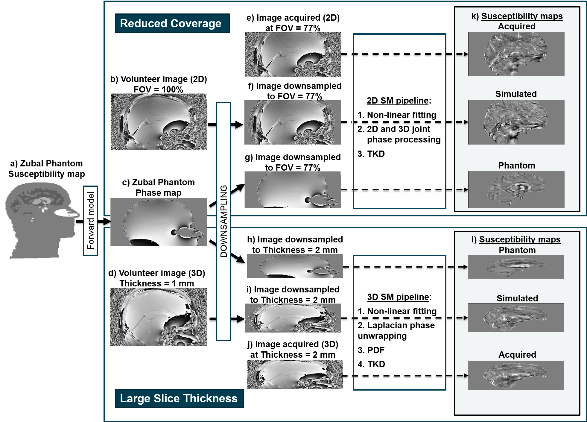
The Zubal head phantom$$$^{11}$$$ was modified: i) to include the neck via co-registration with the torso phantom, ii) by interpolation to achieve 1 mm isotropic resolution, and iii) the oropharyngeal air space was made more realistic using an ellipsoidal shape (Figure 2a). Realistic susceptibility, magnitude and T$$$_2^*$$$ values were assigned to several brain regions$$$^{12}$$$ and a Fourier-based forward model$$$^{13}$$$ was applied to estimate a field map. Multi-echo complex images were simulated at 3-Tesla, TE$$$_1$$$ = 3 ms, $$$\Delta$$$TE = 5.3 ms, 5 echoes (Figure 2c).
Low-resolution complex MRI images were simulated from the full-resolution 3D acquisitions (Figure 2d) and the multi-echo phantom images (Figure 2c) by averaging the complex data across each slab of m = 1 to 6 mm slices (Figure 2h-i). Low-coverage images were simulated from the full-coverage 2D acquisitions (Figure 2b) and the multi-echo phantom images (Figure 2c) by including only the central n = 100% to 14% slices (Figure 2f-g).
Susceptibility maps were calculated from all the 3D and low-resolution images (Figure 2l) using: 1. Non-linear fitting$$$^{14}$$$, 2. Laplacian phase unwrapping$$$^{15}$$$ ($$$\sigma = 10^{-10}$$$), 3. Projection onto Dipole Fields$$$^{16}$$$ (PDF) and 4. Truncated K-space Division$$$^{17}$$$ (TKD, $$$\delta = 2/3$$$, with correction for underestimation$$$^{15}$$$). The same pipeline was applied to the 2D and low-coverage images with steps 2-3 replaced with joint 2D+3D phase processing$$$^{18}$$$ (Figure 2k). Brain masks were generated by combining (by intersection) the result of FSL BET$$$^{19}$$$ on the last-echo magnitude image, and a mask obtained by thresholding the inverse noise map output by the non-linear fit$$$^{20}$$$.
Brain ROIs were obtained via: i) non-rigid registration$$$^{21}$$$ of the Eve atlas$$$^{22}$$$ magnitude image and the full-resolution, full-coverage last-echo magnitude images, ii) the full-resolution, full-coverage susceptibility maps were co-registered$$$^{23}$$$ with all other susceptibility maps and these transformations were applied to the ROIs from the step i). Mean susceptibilities were calculated in several brain regions (referenced to the posterior limb of the internal capsule$$$^{24}$$$ and the internal capsule for the volunteer and phantom respectively).
Results and Discussion
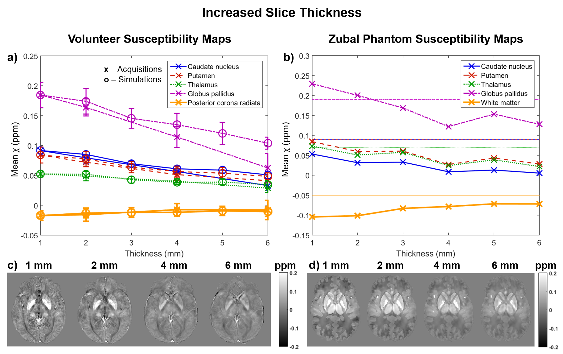
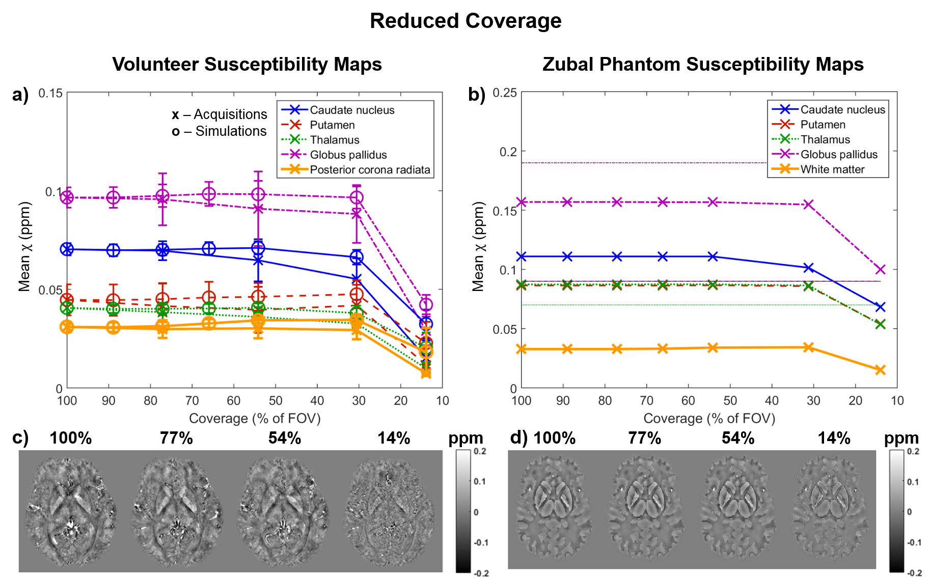
Figures 3 and 4 show the mean susceptibility in several brain regions as a function of slice thickness and coverage respectively for the volunteers (Figures 3a & 4a display both acquisitions (x) and simulations (o)) and the phantom (Figures 3b & 4b). Simulated susceptibility maps in both the volunteers and the phantom were similar to maps from acquired images. The susceptibility map contrast decreased with increasing slice thickness (see Figure 3). Figure 4 suggests that susceptibility maps were not affected by decreased contrast until coverage was reduced below 30% of the FOV (44 mm). The reduced contrast at both increased slice thickness and very low coverage is probably caused by insufficient sampling of the dipolar fields induced by the susceptibility sources. The phantom simulations also show that insufficient sampling leads to incorrect susceptibility values (Figures 3b & 4b where the ground truth values are indicated by the horizontal lines). The mean susceptibilities calculated in the full-coverage, full-resolution images depend on the SM pipeline (see Figures 3b & 4b: The susceptibilities estimated at full resolution/coverage are different for the 3D and 2D pipelines). However, the observed trends suggest that all pipelines would also produce inaccurate results at low resolution and very low coverage.Conclusions
Large slice thickness and very low coverage lead to loss of contrast and errors in susceptibility maps. Resolution and field of view need to be chosen to adequately sample the fields generated by the structures of interest. Simulated susceptibility maps were very similar to maps from acquired images. As calculated susceptibilities depend on the SM pipeline, future work may involve investigating different pipelines.Acknowledgements
This work is supported by the EPSRC-funded UCL Centre for Doctoral Training in Medical Imaging (EP/L016478/1) and the Department of Health’s NIHR-funded Biomedical Research Centre at University College London Hospitals.References
1. J R Reichenbach, F Schweser, B Serres and A Deistung. Quantitative susceptibility mapping: concepts and applications. Clinical neuroradiology. 2015
2. Y Wang and T Liu. Quantitative susceptibility mapping (QSM): decoding MRI data for a tissue magnetic biomarker. Magnetic Resonance in Medicine. 2015
3. C Tudisca, D Price, M Forster, H Fitzke and S Punwani. Exploration of change of T2* of metastatic and normal cervical lymph nodes caused by 100% oxygen breathing. Proc. Intl. Soc. MRM, 2014
4. X Guan, M Xuan, Q Gu, P Huang, C Liu, N Wang, X Xu, W Luo and M Zhang. Regionally progressive accumulation of iron in Parkinson's disease as measured by quantitative susceptibility mapping. NMR in Biomedicine. 2016
5. Y Moon, S H Han and W J Moon. Patterns of Brain Iron Accumulation in Vascular Dementia and Alzheimer’s Dementia Using Quantitative Susceptibility Mapping Imaging. Journal of Alzheimer's Disease. 2016
6. D Zhou, J Cho, J Zhang, P Spincemaille and Y Wang. Susceptibility underestimation in a high-susceptibility phantom: Dependence on imaging resolution, magnitude contrast, and other parameters. Magnetic Resonance in Medicine. 2016
7. W Li, C Liu and B Wu. Quantitative Susceptibility Mapping: Pulse Sequence Considerations. 3$$$^{rd}$$$ Workshop on MRI Phase Contrast and QSM, Durham, North Carolina. 2013
8. E M Haacke, S Liu, S Buch, W Zheng, D Wu and Y Ye. Quantitative susceptibility mapping: current status and future directions. Magnetic Resonance Imaging. 2015
9. A M Elkady, H Sun and A H Wilman. Importance of extended spatial coverage for quantitative susceptibility mapping of iron-rich deep gray matter. Magnetic Resonance Imaging. 2016
10. A Karsa, E Biondetti, S Punwani and K Shmueli. The effect of large slice thickness and spacing and low coverage on the accuracy of susceptibility mapping. Proceedings of the 24th Annual Meeting of the ISMRM, Singapore. 2016
11. I G Zubal, C R Harrell, E O Smith, A L Smith and P Krischlunas. Two dedicated software, voxel-based, anthropomorphic (torso and head) phantoms. In Proceedings of the International Workshop, National Radiological Protection Board, Chilton, UK. 1995
12. E Biondetti, A Karsa, D L Thomas and K Shmueli. The Effect of Averaging the Laplacian-Processed Phase over Echo Times on the Accuracy of Local Field and Susceptibility Maps. 4$$$^{th}$$$ Workshop on MRI Phase Contrast and QSM, Graz, Austria. 2016
13. J P Marques and R Bowtell. Application of a Fourier-based method for rapid calculation of field inhomogeneity due to spatial variation of magnetic susceptibility. Concepts Magn. Reson. B. 2005
14. T Liu, C Wisnieff, M Lou, W Chen, P Spincemaille and Y Wang. Nonlinear formulation of the magnetic field to source relationship for robust quantitative susceptibility mapping. Magnetic Resonance in Medicine. 2013
15. F Schweser, A Deistung, K Sommer and J R Reichenbach. Toward Online Reconstruction of Quantitative Susceptibility Maps: Superfast Dipole Inversion. Magnetic Resonance in Medicine. 2013
16. T Liu, I Khalidov, L de Rochefort, P Spincemaille, J Liu, A J Tsiouris and Y Wang. A novel background field removal method for MRI using projection onto dipole fields (PDF). NMR in Biomedicine. 2011
17. K Shmueli, J A de Zwart, P van Gelderen, T-Q Li, S J Dodd and J H Duyn. Magnetic Susceptibility Mapping of Brain Tissue In Vivo Using MRI Phase Data. Magnetic Resonance in Medicine. 2009
18. H Wei, Y Zhang, E Gibbs, N K Chen, N Wang and C Liu. Joint 2D and 3D phase processing for quantitative susceptibility mapping: application to 2D echo-planar imaging. NMR in Biomedicine. 2016
19. S M Smith. Fast robust automated brain extraction. Human Brain Mapping. 2002
20. MEDI toolbox: http://weill.cornell.edu/mri/pages/qsm.html
21. NiftyReg: http://cmictig.cs.ucl.ac.uk/wiki/index.php/NiftyReg_Segmentation_Propagation_Tutorial
22. I A L Lim, A V Faria, X Li, J T Hsu, R D Airan, S Mori and P C van Zijl. Human brain atlas for automated region of interest selection in quantitative susceptibility mapping: application to determine iron content in deep gray matter structures. Neuroimage. 2013
23. Intensity-based image registration tool in Matlab: https://uk.mathworks.com/help/images/ref/imregister.html
24. S Straub, T M Schneider, J Emmerich, M T Freitag, C H Ziener, H P Schlemmer, M E Ladd and F B Laun. Suitable reference tissues for quantitative susceptibility mapping of the brain. Magnetic Resonance in Medicine. 2016
Figures