3674
Coherence Enhancement in QSM via Anisotropic Weighting in Morphology-Enabled Dipole Inversion1Weill Cornell Medical College, New York, NY, United States, 2Cornell University, Ithaca, NY, United States
Synopsis
The current regularization in morphology-enabled dipole inversion (MEDI) does not take into account orientation information in morphology between QSM and its corresponding magnitude image. In this abstract, we consider such orientation information to enhance structural coherence between the two images. In doing so, we achieve better image quality as well as higher RMSE (root mean square error) and HFEN (high frequency error norm) with respect to COSMOS and $$$\chi_{33}$$$.
Purpose
We focus on the regularization term in morphology-enabled dipole inversion (MEDI). Currently, MEDI makes use of binary-valued isotropic weighting in its regularization so that orientation information in morphology between the magnitude image and QSM has not been carefully considered. Here, we take into account such orientation information by incorporating anisotropic weighting based on the concept of orthogonal projection.Theory
1) Regularized Field-to-Susceptibility Inversion with Isotropic Weighting
In a spatially continuous setting, the problem of regularized dipole inversion is written as follows:
$$ \text{Find } \hat \chi \text{ such that } \hat \chi \in \operatorname{Argmin}\left\{\chi \in BV(\Omega; \mathbb{R}): R(\chi)+ \frac{\lambda}{2}\int_\Omega |w(d*\chi-b)|^2\right\},$$
where the susceptibility distribution $$$\chi:(\Omega \subset \mathbb{R}^3) \to \mathbb{R}$$$ is estimated from the measured local field $$$b:\Omega \to \mathbb{R}$$$. The space of bounded variation, $$$BV(\Omega;\mathbb{R})$$$, allows the existence of jumps modeling sharp edges. The map $$$w:L^1 \to L^1$$$ compensates for the non-uniform phase noise (SNR weighting). The regularization term $$$R(\chi)$$$ is designed in such a way that it effectively penalizes streaking artifacts originated from the dipole-incompatible part of the field (1). Incorporating morphology information extracted from the corresponding magnitude image, the regularization has been typically designed in the following fashion (2):
$$R_{iso}(\chi) := \int_\Omega ||M_G\nabla \chi||_1 = \int_\Omega \left\| \left( \begin{array}{ccc} 1-\delta_{11} & 0 & 0 \\ 0 & 1-\delta_{22} & 0 \\ 0 & 0 & 1-\delta_{33} \\ \end{array} \right) \left( \begin{array}{c} \partial_x \chi \\ \partial_y \chi \\ \partial_z \chi \\ \end{array} \right) \right\|_1,$$
where $$$\delta_{ii}$$$ is an edge indicator function: $$$\delta_{11}(r)=1$$$ if there exists an edge along the x direction; otherwise 0. Likewise, $$$\delta_{22}(r)$$$ and $$$\delta_{33}(r)$$$ are edge indicators along the y and z directions. Therefore, for an edge indicator function determined by the magnitude image, $$$R_{iso}$$$ penalizes only the regions where tissue structure (edges) is not expected.
2) Regularization via Anisotropic Weighting
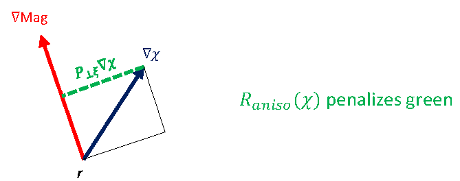
Taking into account orientation information, we expect further improvements in QSM. We modify the regularization term such that it penalizes the perpendicular components of the gradient of susceptibility distribution with respect to the direction of the edges of magnitude image as follows:
$$R_{aniso}(\chi) := \int_\Omega ||P_{\perp\xi}\nabla \chi||_1 = \int_\Omega \left\|\left(I-\frac{\xi\xi^\top}{\xi^\top\xi} \right)\nabla\chi\right\|_1 = \int_\Omega \left\| \left( \begin{array}{ccc} 1-\xi_1^2 & -\xi_1\xi_2 & -\xi_1\xi_3 \\ -\xi_2\xi_1 & 1-\xi_2^2 & -\xi_2\xi_3 \\ -\xi_3\xi_1 & \xi_3\xi_2 & 1-\xi_3^2 \\ \end{array} \right) \left( \begin{array}{c} \partial_x \chi \\ \partial_y \chi \\ \partial_z \chi \\ \end{array} \right) \right\|_1,$$
where $$$\xi$$$ is the gradient of magnitude image, i.e., $$$\xi=\nabla\text{Mag}$$$. In other words, we replace the isotropic weighting $$$M_G$$$ with the orthogonal projector $$$P_{\perp\xi}$$$. We illustrate this in Fig. 1.
Methods
We used two in vivo brain MRI dataset that include COSMOS and as reference:
1. QSM 2016 Reconstruction Challenge
- http://www.neuroimaging.at/qsm2016/pages/qsm-challenge.php
- Both $$$\chi_{33}$$$ and COSMOS are available.
2. Cornell MRI research lab
- http://weill.cornell.edu/mri/pages/qsmreview.html
- COSMOS is available.
We refer the reader to the webpages for more details on data acquisition and phase processing. Computed susceptibility maps were validated against the gold standard ($$$\chi_{33}$$$ or COSMOS) using global metrics: RMSE (root mean squared error), HFEN (high frequency error norm), and SSIM (structure similarity index).
Results
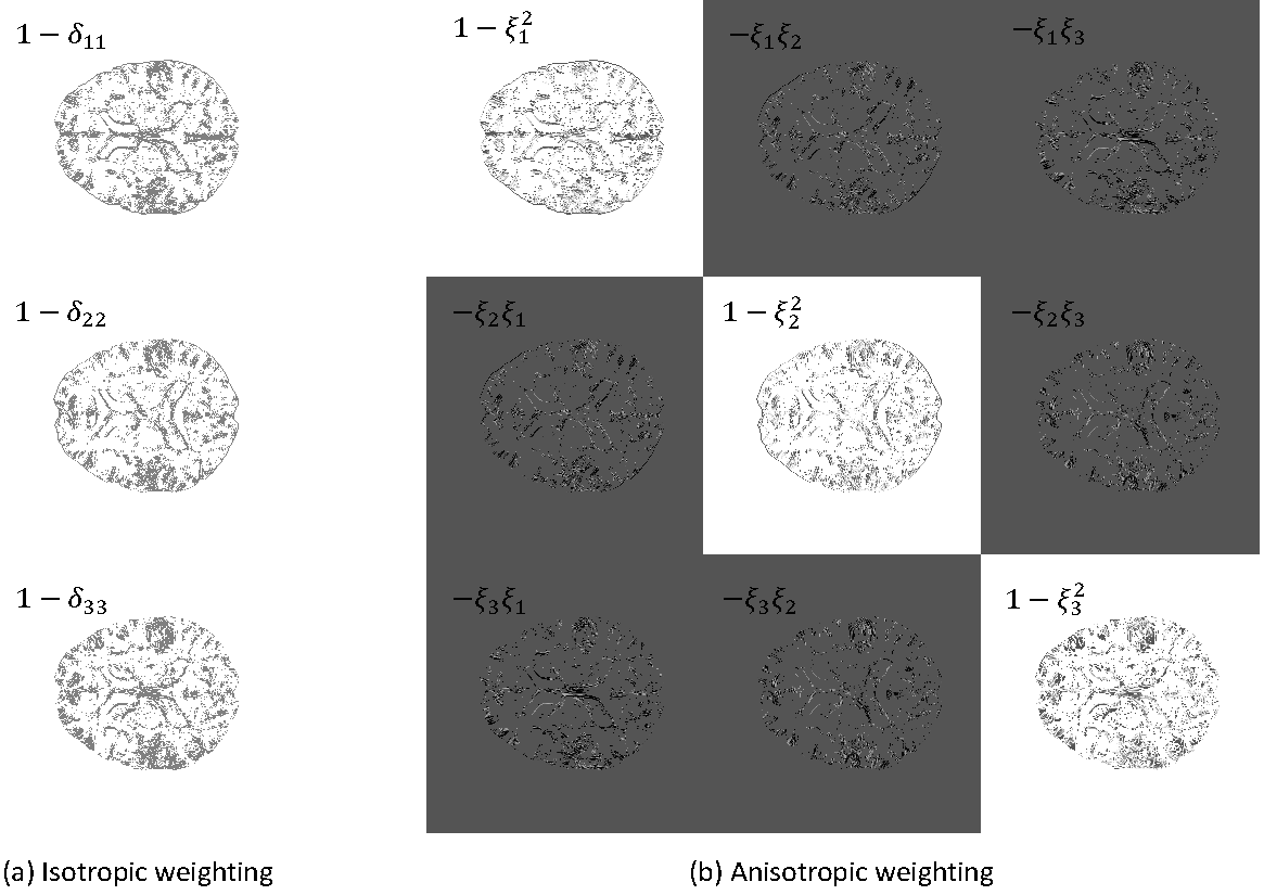
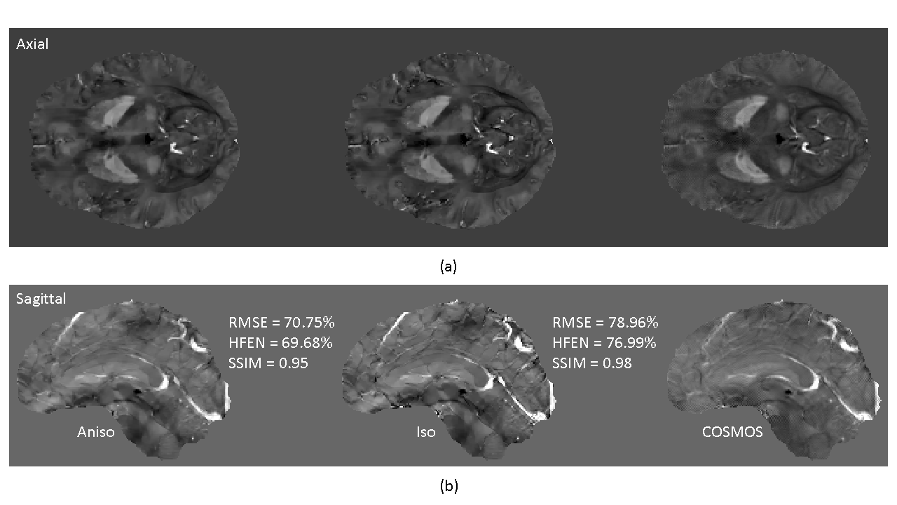
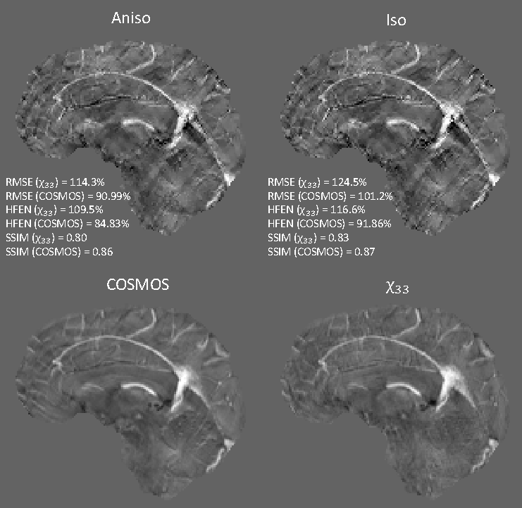
In Fig. 2, we visualize the diagonal components of the isotropic weighting $$$M_G$$$ and the diagonal + off-diagonal components of the anisotropic weighting $$$P_{\perp\xi}$$$. Figs. 3 and 4 show computed susceptibility distributions using MEDI with isotropic/anisotropic weighting.Discussion
As can be seen in Figs. 3 and 4, anisotropic weighting achieved improvements in image quality as well as two quantitative measures – RMSE (root mean square error) and HFEN (high frequency error norm). Visually, this is observed from both axial and sagittal planes in Fig. 3. Notice that black/white dots in isotropic weighting were substantially removed in anisotropic weighting with respect to COSMOS. Although the difference between the two images in FIG. 4 is subtle, similar improvements were observed in anisotropic weighting.
The performance of anisotropic weighting largely depends on a predefined edge indicator function. For the experimental results reported herein, we used the same edge indicator as the isotropic weighting and assigned values in the range of [-1, 1] rather than 1 on the location of edges based on the definition of $$$R_{aniso}(\chi)$$$ described in the Theory section. Therefore, further improvements are expected if the location of edges is optimally estimated.
Anisotropic weighting, on the other hand, has lower values of SSIM (structure similarity index) than isotropic weighting although exhibiting less amount of spurious noise as opposed to isotropic weighting. This will be future research directions.
Conclusion
We have incorporated anisotropic weighting into MEDI in order to take into account morphology in orientation between the magnitude image and QSM. Hence, we were ab le to achieve visual improvements in image quality as well as RMSE and HFEN.Acknowledgements
This research was supported by R01NS072370, R01NS090464, and R01NS095562.References
(1) Choi J. K, Zhou L, Seo J. K, Wang Y. Dipole-Incompatible Field Data Causes Streaking Artifacts in the Field-to-Susceptibility Inverse Problem and Implications for QSM Algorithm Design. QSM Workshop 2016.
(2) Liu J, Liu T, de Rochefort L, Ledoux J, Khalidov I, Chen W, Tsiouris AJ, Wisnieff C, Spincemaille P, Prince MR, Wang Y. Morphology enabled dipole inversion for quantitative susceptibility mapping using structural consistency between the magnitude image and the susceptibility map. Neuroimage 2012;59(3):2560-2568
Figures