Synopsis

We provide a mathematical understanding for artifacts in QSM, particularly streaking artifacts. 1) The local field data can be decomposed into a dipole-compatible part and a dipole-incompatible part. 2) In spatially continuous space, the streaking-free susceptibility solution is obtained from the dipole-compatible field data only, and the dipole-incompatible data leads to artifacts defined by a wave propagator with z as time, specifically, streaking artifacts from granular noise and shadow artifacts from white matter noise error. Although it is not known how to filter out such dipole-incompatible data, its artifacts can be suppressed in regularization-based Bayesian methods such as MEDI, which can efficiently penalize streaking artifacts. k-space-truncation-based methods that generate additional dipole-incompatible data near the zero cone amplify streaking artifacts.

Purpose

Theory

Most QSM algorithms are based on minimizing a cost function that fits the measured tissue magnetic field $$$b({\bf\,r})$$$ (in unit B0) to the dipole field $$$d({\bf\,r})=\frac{2z^2-x^2-y^2}{4\pi|{\bf\,r}|^5},\,\,\mbox{with position vector}\,\,{\bf r}=(x,\,y,\,z)$$$, approximating noise in $$$b$$$ as Gaussian as follows:$$\int_{\mathbb{R}^3}w({\bf\,r})|(d\ast\chi)({\bf\,r})-b({\bf\,r})|^2d{\bf\,r}:=||d\ast\chi-b||_{w}^2.\qquad\quad (1)$$This integral form allows us to estimate the underlying susceptibility distribution with various types of regularization methods. As known from Maxwell’s equations, the integral form represents the solution of the corresponding partial differential equation (PDE):$$\left(\partial_z^2-\frac{1}{2}(\partial_x^2+\partial_y^2)\right)\chi=\frac{3}{2}\Delta\,b,\,\qquad\quad (2)$$which may offer useful insights on a mathematical analysis of susceptibility. This PDE is a wave equation w.r.t. susceptibility $$$\chi$$$ (z-axis is time) and a Laplacian equation w.r.t. field $$$b$$$.

In a spatially continuous setting, we have proved the following two propositions:

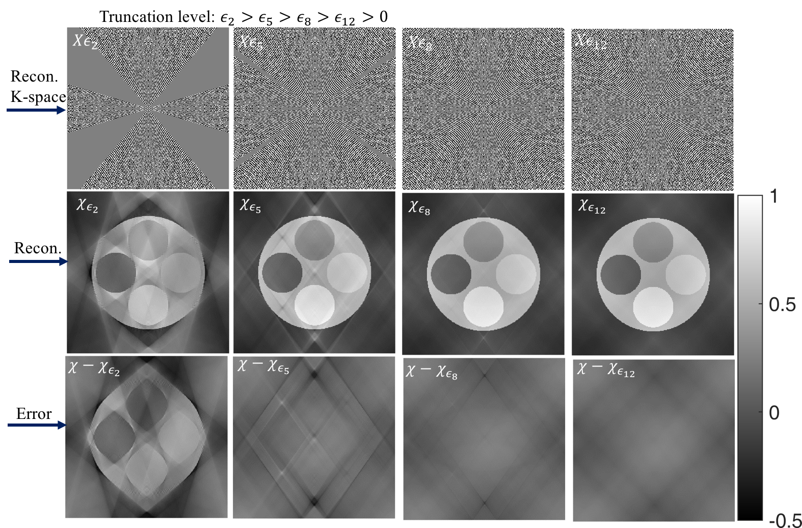
Proposition 1. Non-streaking solution for the dipole-compatible field data: Without any error with $$$b({\bf\,r})=(d\ast\chi)({\bf\,r}), B({\bf\,k})=D({\bf\,k})X({\bf\,k}),$$$ a precise solution of no streaking can be obtained:$$ \chi=\lim_{\epsilon\searrow0}\mathcal{F}^{-1}((1-\eta_{\epsilon})(B/D)).\quad\eta_{\epsilon}=1\,\,\mbox{ if }\,|D({\bf k})|<\epsilon\,\,\mbox{otherwise}\,\,0.\qquad\quad(3)$$

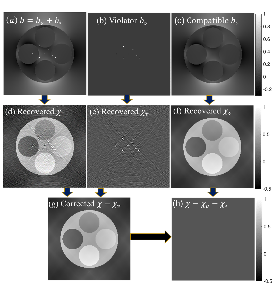
Proposition 2. Streaking solution for the dipole-incompatible field data: Any$$$\,$$$field data that cannot be fitted to the dipole field is referred to as the dipole-incompatible field$$$\,$$$data $$$v({\bf\,r})$$$, which may come from various causes including discretization error, noise, and anisotropy sources. The granular noise in the dipole-incompatible data causes streaking artifacts according to the wave propagation solution:$$\chi_v({\bf\,r})=-\int G({\bf\,r},{\bf\,r}')\cdot\frac{3}{2}\Delta v({\bf\,r}')d{\bf\,r}'\,\mbox{with}\,G({\bf\,r},{\bf\,r}'):=\frac{1}{2\pi\sqrt{(z-z')^2-2((x-x')^2+(y-y')^2)}}>0,\qquad\quad(4)$$where $$$G({\bf\,r},{\bf\,r}')$$$ defines magic-angle cones above and below the incompatible source $$$\frac{3}{2}\Delta v({\bf\,r}')$$$. Strong streaking exhibits along the cone surface where $$$G({\bf\,r},{\bf\,r}')$$$ is large; the streaking manifests as streaking in saggital and coronal view, but as ringing in axial view. It is noted that the contiguous anisotropy sources (e.g. brain white matter) as a modeling error contribute to the dipole-incompatible$$$\,$$$field$$$\,$$$data, which may result in shadow-like artifacts according to Eq.$$$\,$$$(4).

Methods

We generated a numerical phantom to demonstrate the two propositions: First, we demonstrated the fact that a precise$$$\,$$$(non-streaking)$$$\,$$$solution can be obtained as $$$\epsilon\rightarrow0$$$ in Eq.$$$\,$$$(3)$$$\,$$$in$$$\,$$$Proposition$$$\,$$$1. Second, we generated dipole-incompatible$$$\,$$$field$$$\,$$$data$$$\,$$$(violators)$$$\,$$$and demonstrated theirs wave propagation solutions, i.e., streaking artifacts.

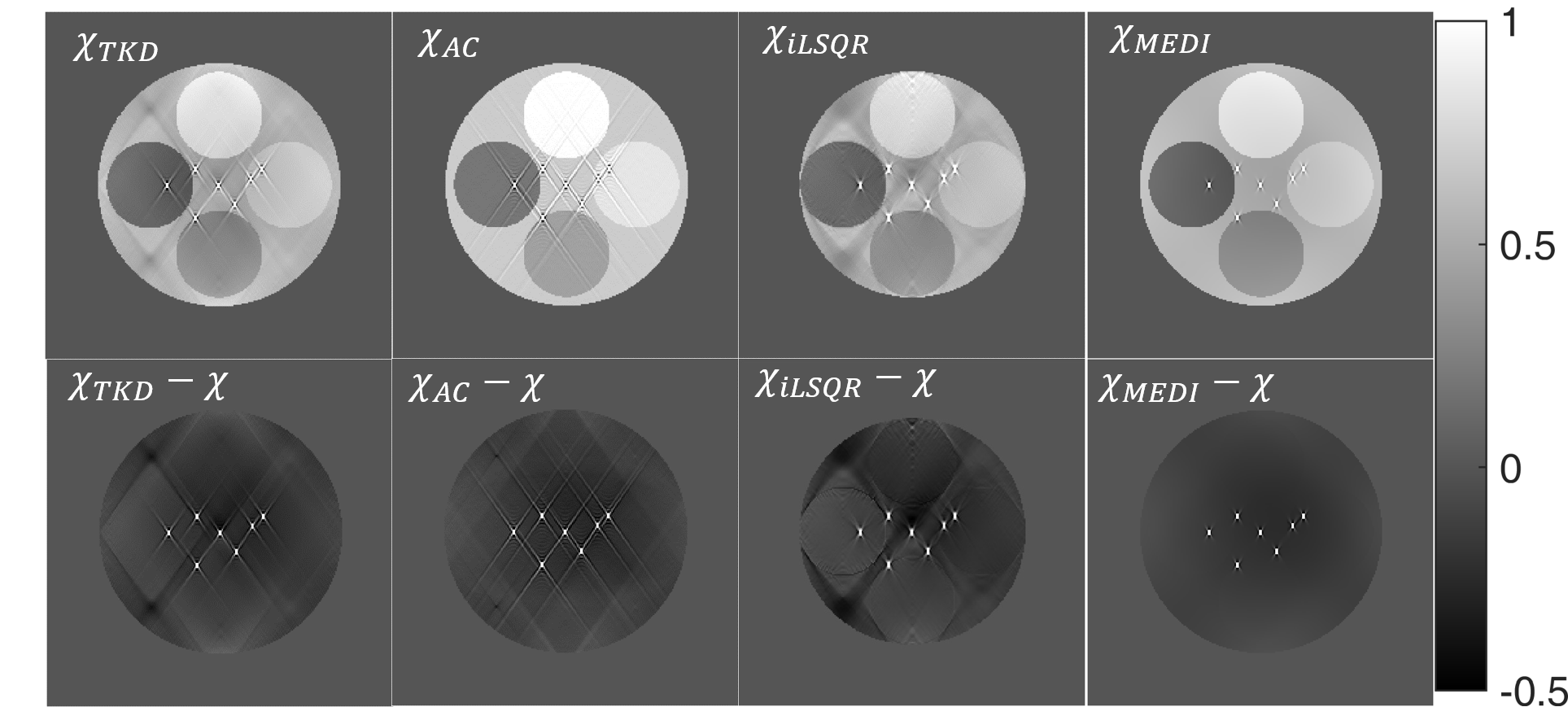
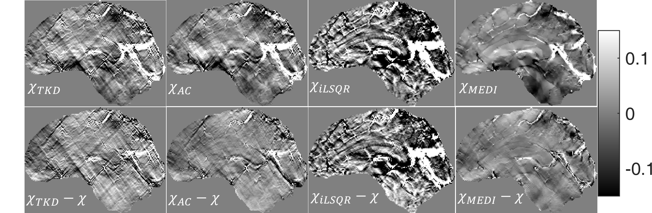
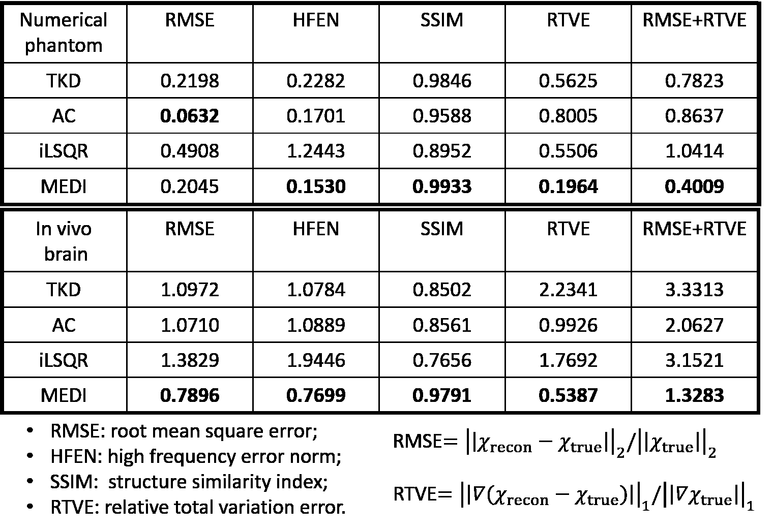
We compared the performance of TKD¹, AC², iLSQR³ and MEDI⁴ on the numerical phantom and in vivo brain MRI data.

Results

Fig.$$$\,$$$1 shows the demonstration of Proposition 1. Fig.$$$\,$$$2 shows the wave propagation solution of the incompatible data.

Figs.$$$\,$$$3$$$\,$$$and$$$\,$$$4 illustrate the performances of TKD, AC, iLSQR and MEDI on phantom and in vivo brain data,$$$\,$$$respectively. The performance metrics are summarized on Table.$$$\,$$$1, suggesting that MEDI is preferable in reducing streaking artifacts.

Discussion

The$$$\,$$$above$$$\,$$$two$$$\,$$$propositions may explain the streaking artifacts observed in various QSM results: Errors in experimental data are omnipresent, including noise, anisotropy sources and digitization errors. Therefore, Eq.$$$\,$$$(1) alone will invariably result in streaking artifacts. Obviously, streaking artifacts can be avoided by extracting the dipole-compatible part of the$$$\,$$$field$$$\,$$$data only. However, the existence of such a decomposition method$$$\,$$$(furthermore$$$\,$$$its$$$\,$$$practicability)$$$\,$$$is yet to be established. Note$$$\,$$$that$$$\,$$$in$$$\,$$$Fig.$$$\,$$$1,$$$\,$$$we$$$\,$$$started$$$\,$$$with$$$\,$$$the$$$\,$$$dipole-compatible$$$\,$$$field$$$\,$$$data$$$\,$$$only,$$$\,$$$but$$$\,$$$the$$$\,$$$discretization$$$\,$$$introduced$$$\,$$$the$$$\,$$$dipole-incompatible data$$$\,$$$near$$$\,$$$the$$$\,$$$zero$$$\,$$$cone$$$\,$$$and$$$\,$$$consequent$$$\,$$$streaking$$$\,$$$artifacts.

Algorithmically, streaking artifacts can be substantially suppressed by penalizing their unique properties. Streaking appears along the magic angle$$$\,$$$(54.7⁰),$$$\,$$$making it distinct from the tissue edges⁵. Hence, tissue structure information can be used to identify a solution of minimal streaking, which is the morphology enable dipole inversion (MEDI) approach². The MEDI method penalizes the sum of the gradients of susceptibility across the image volume in terms of the L1-norm except for the locations where tissue edges are expected. Therefore, it effectively reconstructs the tissue edges in susceptibility. The tissue structure information may be incorporated into regularization in various elaborate manners such as in HEIDI⁶, SWIM⁷, CCD⁸ and iLSQR³.

Note that the truncated k-space division¹ (TKD) increases the dipole-incompatible part of the data in certain k-space locations where the truncation causes deviation from the dipole kernel. LSQR⁹ with a few iterations, which has also been used to generate QSM, may be regarded as some kind of truncation in the Krylov subspace; thus suffers from streaking artifacts.

Conclusion

Acknowledgements

References

1. Shmueli K, et al. Magnetic susceptibility mapping of brain tissue in vivo using MRI phase data. Magn Reson Med 2009; 62(6):1510-22.

2. Natterer F, Image reconstruction in quantitative susceptibility mapping. SIAM J Imag Sci 2016; 9(3):1127-1131.

3. Li W, et al. A method for estimating and removing streaking artifacts in quantitative susceptibility mapping. Neuroimage 2015; 108:111-22.

4. de Rochefort L, et al. Quantitative susceptibility map reconstruction from MR phase data using bayesian regularization: validation and application to brain imaging. Magn Reson Med 2010; 63(1):194-206.

5. Wang Y, et al. Quantitative susceptibility mapping (QSM): Decoding MRI data for a tissue magnetic biomarker. Magn Reson Med 2015; 73(1):82-101.

6. Schweser F, et al. Quantitative susceptibility mapping for investigating subtle susceptibility variations in the human brain. Neuroimage 2012; 62(3):2083-100.

7. Tang J, et al. Improving susceptibility mapping using a threshold-based K-space/image domain iterative reconstruction approach. Magn Reson Med. 2013; 69(5):1396-407.

8. Wen Y, et al. Enhancing k-space quantitative susceptibility mapping by enforcing consistency on the cone data (CCD) with structural priors. Magn. Reson. Med 2016; 75(2):823-30.

9. Li W, et al. Quantitative susceptibility mapping of human brain reflects spatial variation in tissue composition. Neuroimage 2011; 55(4):1645-56.