3671
Discrete frequency shift signatures explain GRE-MRI signal compartments1Centre for Advanced Imaging, University of Queensland, St Lucia, Australia
Synopsis
Ultra-high field GRE-MRI phase images present great promise for structural brain studies. Multi-echo GRE-MRI data has been shown to contain signal compartments, which may eventually be used to characterise brain microstructure. Existing studies considered three signal compartments, however it remains unclear how compartments co-localise throughout the brain. We compartmentalised the signal via frequency shift signatures in a mixture of grey-white matter brain regions and implemented quality of fit measures to select the most parsimonious model for each region. We utilised k-means cluster analyses to investigate signal compartment commonalities across different brain regions and found four dominant frequency shift signatures.
Purpose
MRI-based neuroimaging studies have demonstrated the utility of GRE-MRI signal phase in structural brain studies.1 With an inability to advance ultra-high field magnetic resonance image contrast to the micro-scale, there exists an increasing need to resolve information about voxel sub-structures based on millimeter scale measurements. Recent studies suggest that temporal changes in frequency shift and magnetic susceptibility, computed from multi-echo GRE-MRI data, contain information on voxel sub-compartments.2-8 The three-pool, or three-compartment model (comprised of myelin, axonal and an extracellular water signals) has been increasingly employed to investigate neural microstructure.3-8 This approach, however, limits model complexity across brain regions that significantly vary in cytoarchitecture. For example, we recently showed via temporal susceptibility mapping that not only white matter, but also grey matter contain signal compartments.7 It remains unclear whether the three-pool model accurately describes signal compartments for all brain structures. Thereby, our aim is to evaluate the differences in GRE-MRI signal compartments across structurally diverse brain regions.Methods
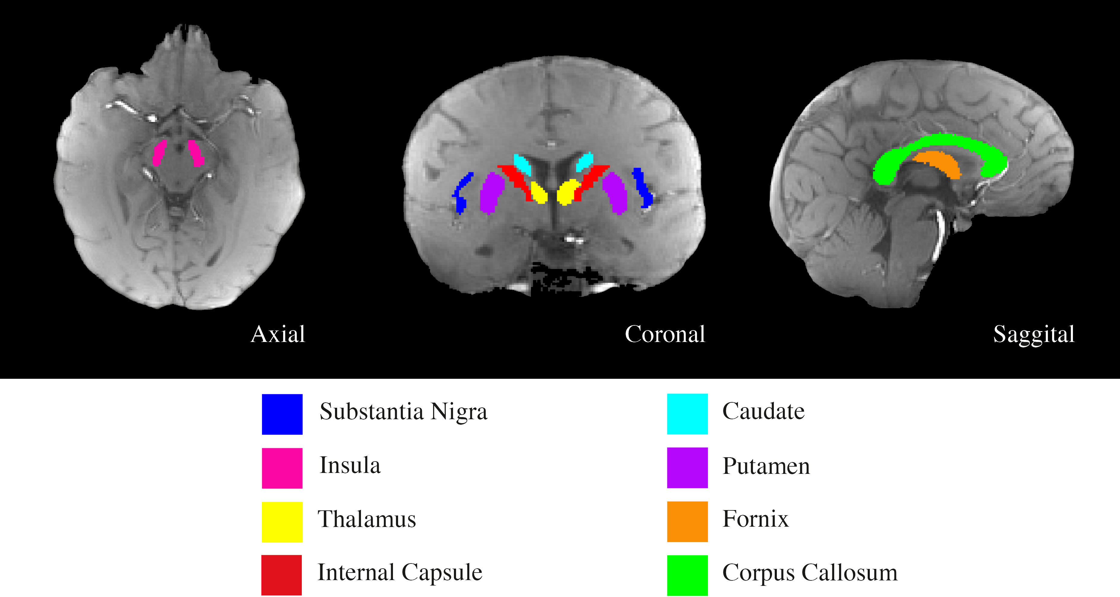
The University of Queensland human ethics committee approved this study and written informed consent was provided by five healthy participants (aged 30 to 41). 3D GRE-MRI non-flow compensated scans were conducted on a 7T ultra-high field whole-body MRI research scanner (Siemens Healthcare, Erlangen, Germany) with a 32 channel dedicated head coil (Nova Medical, Wilmington, USA) using the following parameters: TE1=2.04ms, echo spacing=1.53ms, 30 echoes, TR=51ms, flip angle=15o, voxel size = 1mm$$$\times$$$1mm$$$\times$$$1mm and matrix size = 210$$$\times$$$168$$$\times$$$144. Image processing and region of interest (ROI) segmentation were performed as outlined previously.8 Data were averaged at each echo time for each region across all participants. Brain regions in Fig 1 were compartmentalised using volume fraction An, T2*, and frequency shift ($$$\triangle$$$f), as in previous studies:6,7,8 $$S(t)=\sum_{i=1}^{N}A_ie^{-\frac{t}{T_{2,i}^*}-i2\pi{{\triangle}f_{i}}},N = 1,...,6$$ Since three compartments mostly generate a good fit, we tested a maximum of six compartments to achieve highest model accuracy and avoid over-paramterisation.5-8 Model parameters were obtained using an iterative non-linear least squares regression algorithm (lsqnonlin). The most parsimonious compartment model within each brain region was selected based on the adjusted coefficient of determination (R2) and the Akaike Information Criterion (AIC).9 We implemented k-means cluster and silhouette analyses to identify trends in compartment frequency shift signatures (FSS) between different regions. All scripts were implemented in MATLAB®.Results
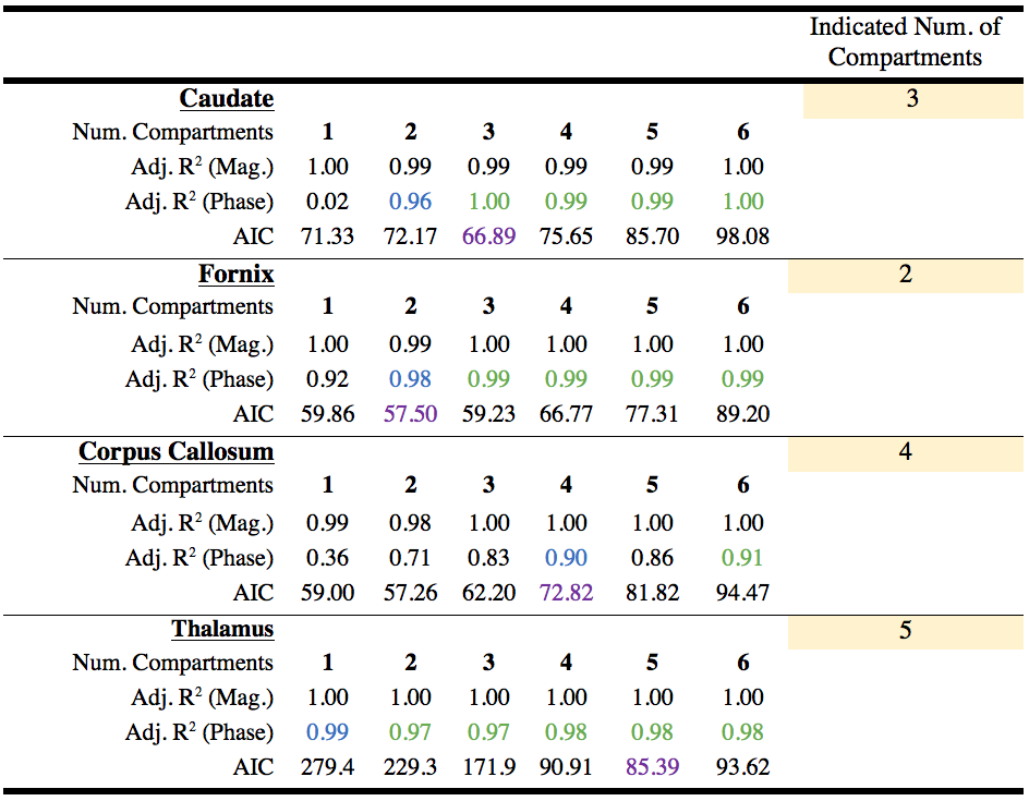
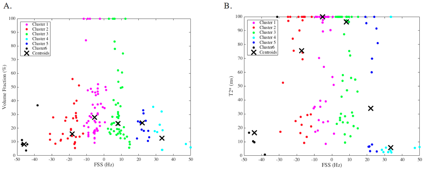
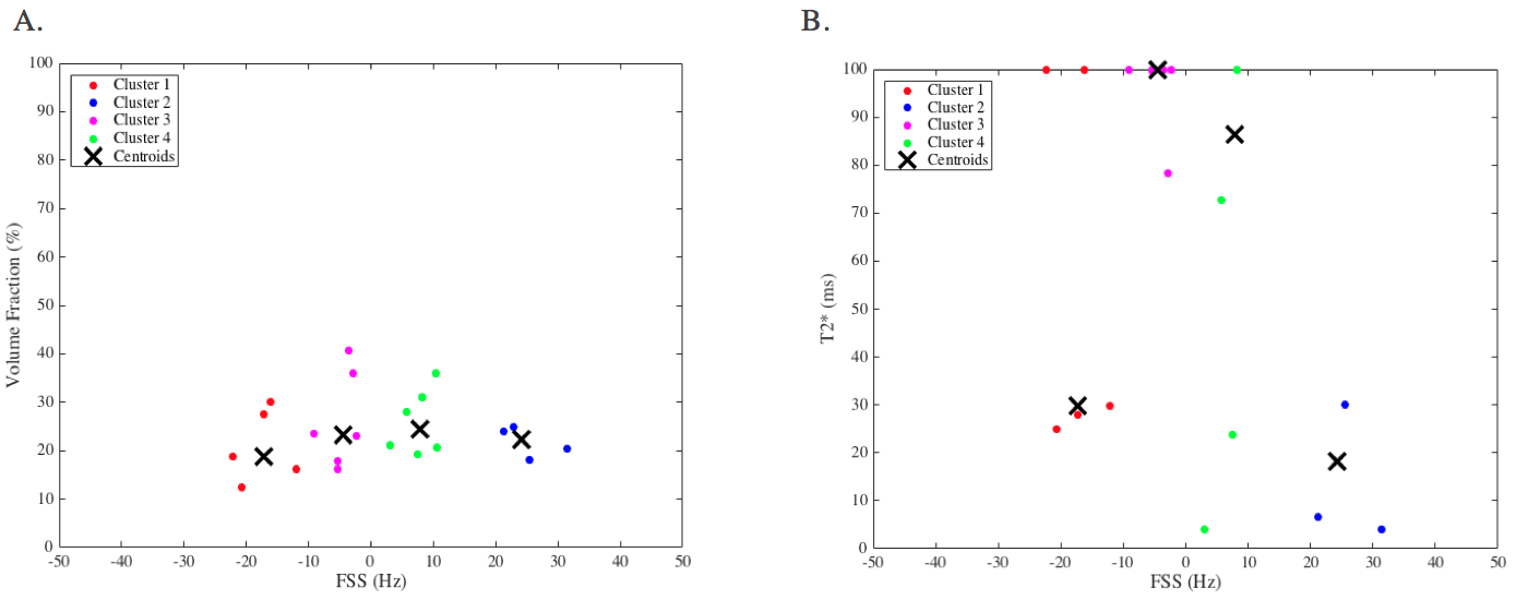
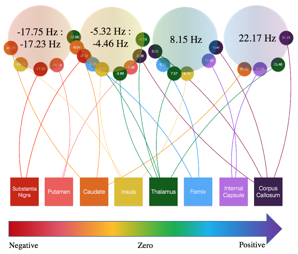
The adjusted R2 and AIC values indicate a varying number of compartments within individual brain regions (Table 1). Fig 2 highlights the six discrete compartment FSS obtained using the cluster analysis based on 1 to 6 compartment models; the centroid of each frequency shift cluster was used to define FSS of the compartment, and minor compartments exhibited a small number of clustered data points. We attributed compartments with a small An and T2* to noise (Fig 2; cluster 6--black points). In a different analysis, we used the AIC criterion to select the best model for each brain region (see Table 1). Fig 3 displays k-means cluster analysis results based on compartment FSS from the best model in each brain region (i.e. dominant compartments only). Interestingly, the FSS centroids for the four compartments in Fig 3 matched within 1.0Hz to the four major compartments in Fig 2. Fig 4 summarises FSS compartments and how they link with different brain regions.Discussion
Results from Fig 2 through Fig 4 elucidate distinct FSS values for signal compartments. Compartment FSS values co-localised at nearly identical centroid values when the AIC was not considered and when the AIC was utilised to restrict the number of model compartments (compare Fig 2 and Fig 3); this suggests four major FSS values that each represent a discrete signal compartment. Table 1 shows that by increasing the number of signal compartments, a better fit of the data was not achieved beyond a certain point, and when additional compartments were considered, FSS values started to repeat. These findings imply distinct and globally representative sources of multi-echo GRE-MRI signals within the investigated brain regions. In Fig 4 we also compared our findings against those by Sati et al. and Li et al;8,10 their findings for myelin water, with an FSS between 20Hz to 25Hz, and axonal water with FSS between -6Hz to -4Hz, closely match two of our major FSS contributors (22.17Hz, and -5.32Hz to -4.46Hz in Fig 4).Conclusion
We observed four major FSS values across grey and white matter regions which broadly validate previous findings based on the three-compartment model. The four compartment FSS identified using our data driven approach may lead to volume fraction maps for distinct signal compartments and promote the use of signal compartments in structural brain studies.Acknowledgements
The authors acknowledge the facilities provided by the National Imaging Facility at the Centre for Advanced Imaging, University of Queensland. The authors also acknowledge funding from the Australian Research Council (DP140103593).References
1. Duyn JH, van Gelderen P, Li TQ, Zwart JA, de Koretsky AP, Fukunaga M. High-field MRI of brain cortical substructure based on signal phase. Proc Natl Acad Sci. 2007;104:11796–11801.
2. Zhong, K, Leupold J, Elverfeldt DV, & Speck O. The molecular basis for gray and white matter contrast in phase imaging. NeuroImage. 2008;40(4):1561-1566.
3. Lancaster JL, Andrews T, Hardies L J, Dodd S, & Fox PT. Three-pool model of white matter. Journal of Magnetic Resonance Imaging. 2002;17(1):1-10.
4. Du YP, Chu R, Hwang D, Brown MS, Kleinschmidt-Demasters BK, Singel D, & Simon JH. Fast multislice mapping of the myelin water fraction using multicompartment analysis of T2* decay at 3T: A preliminary postmortem study. Magnetic Resonance in Medicine Magn. Reson. Med. 2007;58(5):865-870.
5. Hwang D, Kim D, & Du YP. In vivo multi-slice mapping of myelin water content using T2* decay. NeuroImage. 2010;52(1):198-204.
6. Nam Y, Lee J, Hwang D, & Kim D. Improved estimation of myelin water fraction using complex model fitting. NeuroImage. 2015;116:214-221.
7. Sood S, Urriola J, Reutens D, O’Brien K, Bollmann S, Barth M, & Vegh V. Echo time-dependent quantitative susceptibility mapping contains information on tissue properties. Magnetic Resonance in Medicine Magn. Reson. Med. 2016.
8. Sati P, van Gelderen P, Silva AC, et al. Micro-compartment specific T2* relaxation in the brain. NeuroImage. 2013;77:268–278.
9. Akaike H. Akaike’s Information Criterion. International Encyclopedia of Statistical Science. M. Lovric. Berlin, Heidelberg, Springer Berlin Heidelberg. 2011:25-25.
10. Li X, van Gelderen P, Sati P, Zwart JA, Reich DS, Duyn JH. Detection of demyelination in multiple sclerosis by analysis of T2* relaxation at 7T, Neuroimage: Clinical. 2015;7:709-714.
Figures