3670

Effect of Poisson kernel parameters on background field removal accuracy for QSM

Debra E. Horng^1,2, Samir D. Sharma¹, Scott B. Reeder^1,2,3,4,5, and Diego Hernando^1,2

¹Radiology, University of Wisconsin, Madison, WI, United States, ²Medical Physics, University of Wisconsin, Madison, WI, United States, ³Biomedical Engineering, University of Wisconsin, Madison, WI, United States, ⁴Medicine, University of Wisconsin, Madison, WI, United States, ⁵Emergency Medicine, University of Wisconsin, Madison, WI, United States

Synopsis

The Poisson Estimation for Ascertaining Local fields (PEAL) kernel is a recently-introduced method for background field removal in quantitative susceptibility mapping (QSM). The PEAL kernel is determined by two parameters: radius and spatial shift. The choice of these two parameters may have a substantial effect on the accuracy of background field removal. In this work, we assessed the effect of PEAL kernel size and shift on the accuracy of background field removal and susceptibility estimation.

Introduction

Quantitative susceptibility mapping (QSM) is an emerging phase-based magnetic resonance imaging (MRI) method for quantifying local deposition of iron in the body. Accurate assessment of the magnetic susceptibility distribution with QSM requires unwrapping the phase data, removing phase contributions from outside sources (“background field”), and solving the inverse problem that estimates susceptibility from phase data. Current background field removal methods assume that the structures of interest are not located close to tissue-air interfaces. Recently, a new background field technique was proposed,¹ which has the potential to accurately remove the background field in tissue regions close to an air interface. The purpose of this work is to characterize this background field removal method in terms of the effect of kernel size and kernel shift on the accuracy of field map and susceptibility estimation.

Theory

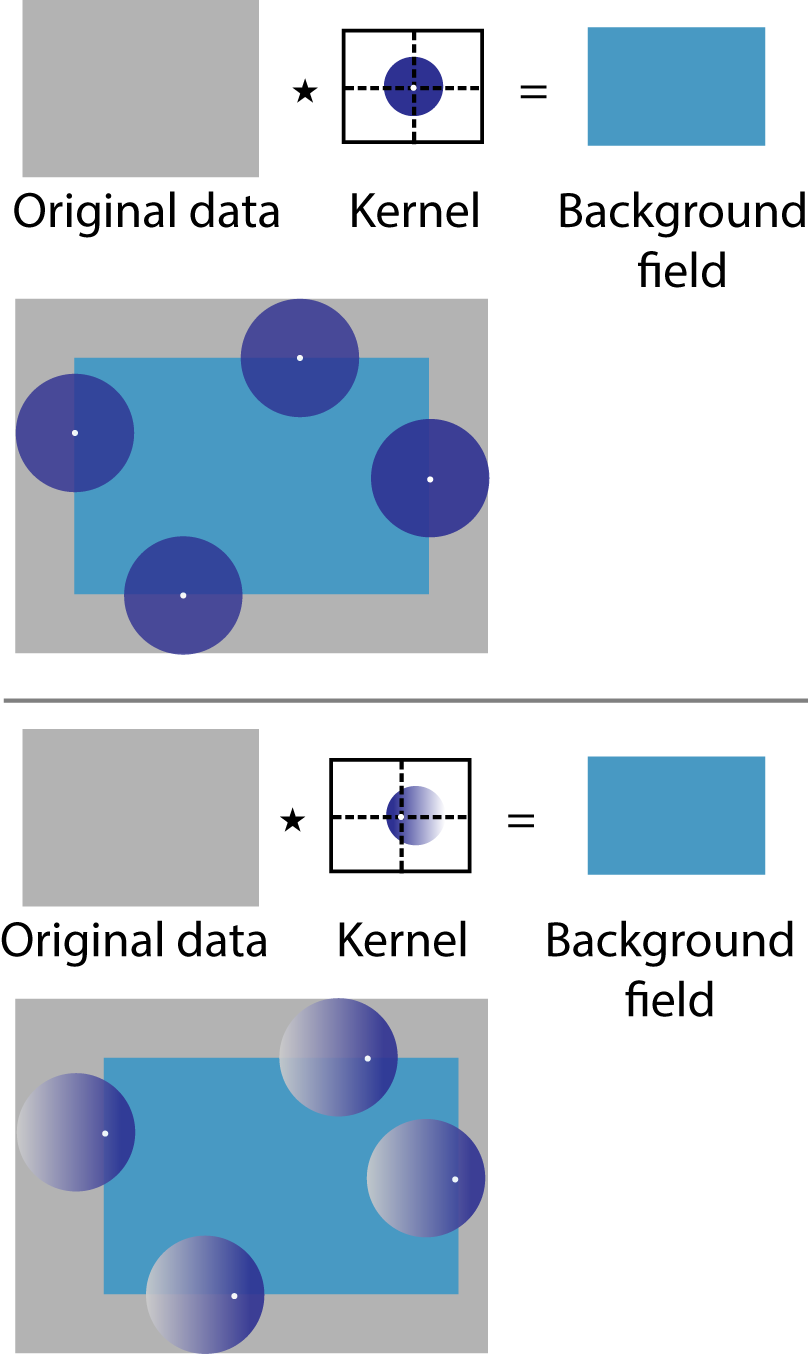
Poisson kernel values within a sphere of radius R at a fixed center $$$\vec{c}$$$ are described by: $$P_{R,\vec{c}}= \frac{R^2[R^4-|\vec{r}-\vec{c}|^2|\vec{c}|^2]}{V[R^4-2R^2(\vec{r}-\vec{c})\cdot\vec{c}+|\vec{r}-\vec{c}|^2|\vec{c}|^2]^{3/2}}\text{ if }|\vec{r}|<R$$ where V is the volume of the sphere. There are many possible kernels for one radius R, depending on the choice of sphere center $$$\vec{c}$$$.

Methods

To examine the accuracy of a particular kernel, we will examine both estimated local fields, and estimated susceptibility values.

Simulation: A digital phantom was created of a cylinder at ‑2.2ppm (“test tube”, diameter 1.4cm, height 6.4cm) in a rectangular prism at -9.02ppm (“water bath”, 12.8cm×12.8cm×6.4cm). The matrix size was 512×512×128 with 1.0mm isotropic resolution and the test tubes were located at both central and edge positions. Synthetic field maps were created^2-4 for both local and background fields.

Phantom: A susceptibility phantom comprised of a polypropylene test tube (diameter 1.6cm, height 7cm) was created with 0, 1, 2, 3, and 4% aqueous dilutions of gadobenate dimeglumine (MultiHance, Bracco Diagnostics, Princeton, NJ, USA). Each test tube was submerged in a rectangular water bath (21.5cm×14.7cm×7cm). The dilutions have calculated susceptibilities of 0.0, 1.7, 3.4, 5.2, and 6.9 ppm respectively, relative to water at 0.0 ppm, chosen to correspond to the range of susceptibilities for liver iron overload that are encountered clinically.⁵

Phantom imaging: Imaging was performed on a 1.5T clinical MRI system (Signa HDxt, GE Healthcare, Waukesha, WI, USA), with an 8-channel phased array torso coil, using a multi-echo 3D spoiled gradient echo (SGRE) sequence. Parameters: no parallel imaging, FOV=25.6 cm, slice=1.0 mm, matrix=128×128, TE1=1.1ms, ΔTE=1.7ms, TR=11.3ms, 6 echoes/TR (flyback readout), flip angle=5°, averages=4, BW=±62.5kHz. Each of the test tubes was scanned at two locations, central and next to an edge. Images were reconstructed at 1.0mm isotropic resolution. The field map was estimated using a per-voxel linear fit of unwrapped phase vs. TE.

Background field removal: For both simulation and phantom data, field maps were processed with PEAL kernels of radii 6 and 12, with kernel shifts from 0-5 (radius 6) and 0-10 (radius 12). The kernel shifts were chosen to be comparable between radius sizes.

Dipole inversion: For both simulation and phantom data, the water bath was assumed to be 0ppm, and one constant susceptibility was estimated for all voxels inside the test tube.

Results

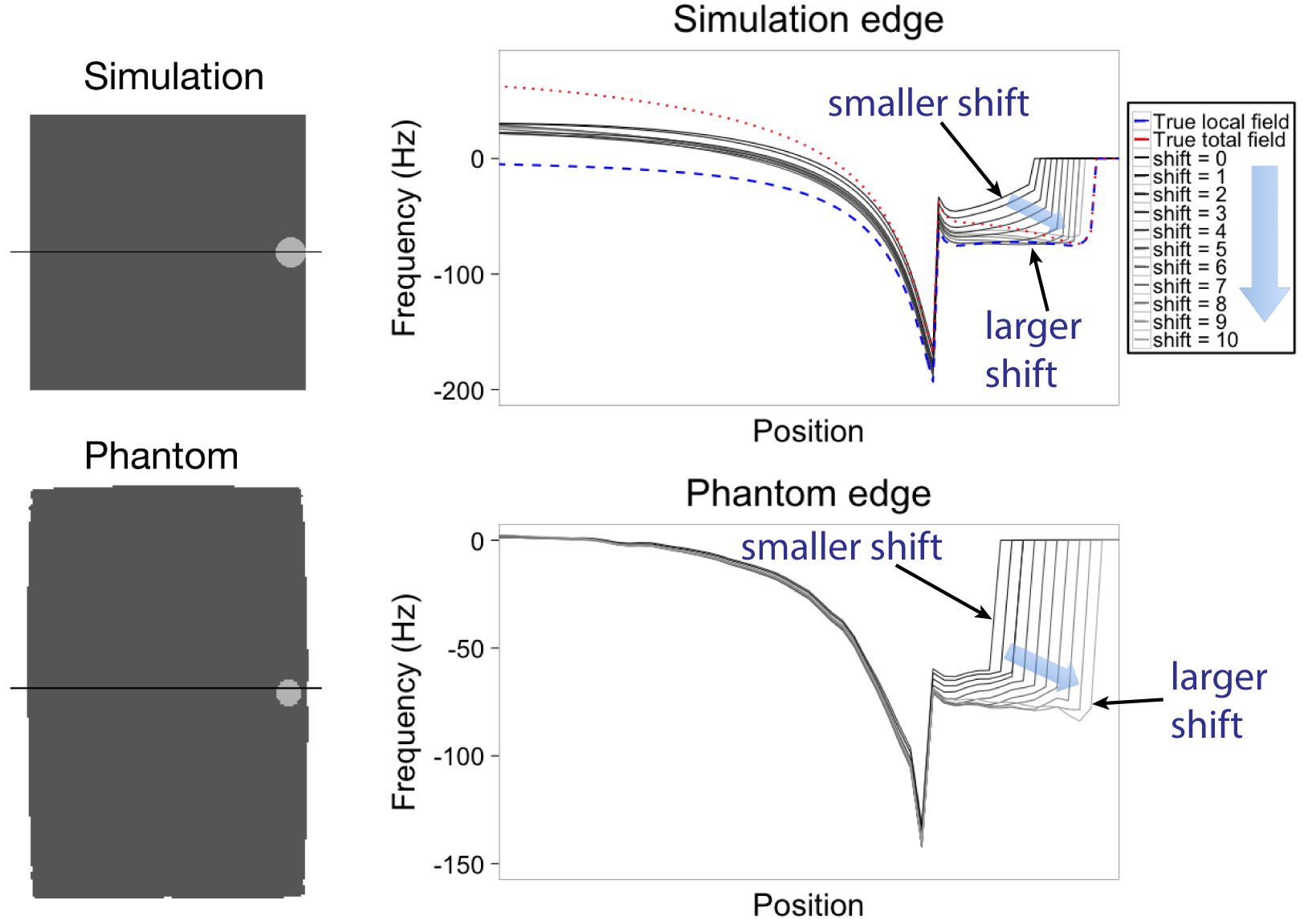
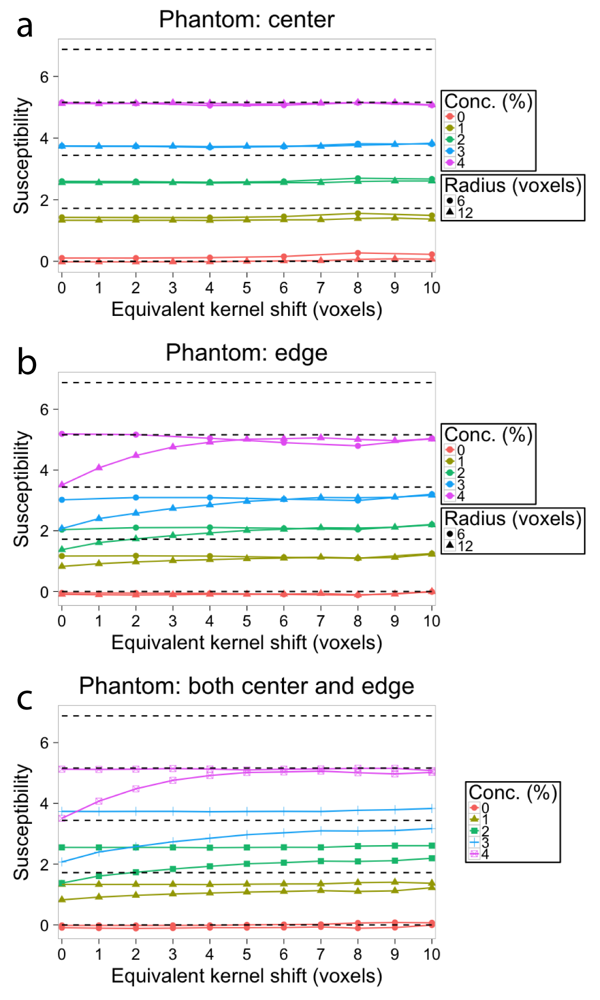
Figure 2 shows the estimated local field for different kernel shifts, and how more edge values are recovered for higher kernel shifts. Figure 3 shows horizontal profiles in the estimated local field data, which shows that larger kernel shift leads to greater accuracy in horizontal profiles of the estimated local field at the edge location. As shown in Figure 4, estimated susceptibility from phantom data is fairly constant across choices of kernel radius and kernel shift, with the exception of the larger kernel (radius=12) combined with the smaller kernel shifts (0-4 voxels). As shown previously for phantom data,⁶ the true susceptibility is underestimated with each concentration.

Discussion and Conclusion

PEAL kernels can enable accurate background field removal near the edge of an object. Kernel size and shift affect the field map values, but do not greatly affect susceptibility estimation, with the exception that larger kernel shifts should be used for larger radius kernels near the edge of an object. This exception may be the result of eroded support area with smaller shifts. Overall, PEAL performance in susceptibility estimation will also depend on the implemented dipole inversion algorithm. In conclusion, a large range of PEAL kernel sizes and shifts are viable choices, without any decrease in susceptibility accuracy.

Acknowledgements

The authors wish to acknowledge support from the NIH (UL1TR00427, R01 DK083380, R01 DK088925, R01 DK100651, and K24 DK102595), as well as GE Healthcare.

References

1. Horng D et al. ISMRM 2016; 29. 2. Salomir R et al. Concept Magnetic Res. 2003; 19B:26-34. 3. Marques JP et al. Concept Magn Reson B. 2005; 25B:65-78. 4. Koch KM et al. Phys Med Biol. 2006; 51:24,6381-402. 5. Schenck JF. Med Phys 1996; 23:815-50. 6. Zhou D et al. MRM 2016; early view.

Figures

Figure 1. Processing the field map with harmonic theory-based kernels leads to spatial erosion. However, the area of support may be moved toward areas of interest with the use of a Poisson kernel. In this example, field map values closer to the right side of the phantom may be recovered.

Figure 2. (Animated.) The area of support in the field map may be moved, depending on the kernel shift. A central slice of the estimated local field from phantom data is shown on the left, and the kernel that was used to implement background field removal is shown on the right. The kernel is spherical; a cutaway is shown, with a black dot to denote the center of convolution space. The kernel shift is the distance from the black dot to the center of the sphere.

Figure 3. Larger kernel shift leads to greater accuracy in the estimated local field at the edge location. The field maps processed with PEAL kernels of radius=12 and different shifts show greater accuracy at the edge for higher kernel shifts. In simulation, horizontal profiles at the edge location show that the larger kernel shifts (lighter gray lines) are closer to the blue dashed profile of the true local field. In the phantom, the higher kernel shifts show the same pattern. In the center location (not shown), simulation and phantom profiles are similar regardless of this horizontal kernel shift.

Figure 4. (a.) When the test tube is at the center location, radius and shift of the PEAL kernel do not substantially affect the estimated susceptibility. The curves are flat across all kernel shifts. (b.) If the test tube is at the edge location, the smaller kernel shifts (0-4) in the larger kernel (radius=12) lead to more inaccurate susceptibility estimates. (c.) Both center and edge locations are shown for the larger kernel (radius=12). For all plots, the true susceptibilities are shown by dashed black lines.

Proc. Intl. Soc. Mag. Reson. Med. 25 (2017)

3670