3669
A Fast Algorithm for Nonlinear QSM Reconstruction1Electrical Engineering, Pontificia Universidad Catolica de Chile, Santiago, Chile, 2Biomedical Imaging Center, Pontificia Universidad Catolica de Chile, Santiago, Chile, 3Martinos Center for Biomedical Imaging, Harvard Medical School, MA, United States, 4German Center for Neurodegenerative Diseases (DZNE), Magdeburg, Germany
Synopsis
This abstract presents a fast nonlinear solver for the QSM reconstruction using the total generalized variation regularization. The proposed method utilizes the alternating direction method of multipliers to obtain close-form solution to each sub-problem. To handle the non-linear data fidelity, a two-step algorithm is described, including a global optimum search and a local Newton-Raphson iteration. Compared to conventional linear solvers, nonlinear solutions reduce streaking artifacts and better handle noise in poor SNR regions. Reconstruction results are at least comparable to nonlinear MEDI in quality, but with an order of magnitude improvement in the computational efficiency.
PURPOSE
Quantitative Susceptibility Mapping (QSM) inversion is often performed through a minimization of a energy functional consisting of a regularization and data fidelity terms. The data fidelity term comprises a susceptibility-to-field relationship based on a phase noise distribution. While such a distribution can be approximated by a Gaussian function in most cases, it often breaks down when SNR becomes low [1]. To address this issue, Liu et al. [2] proposed a nonlinear data fidelity term based on a phase projection into the complex image domain. An exhaustive comparison of noise models [3] showed the benefits of using such non-linear formulation, i.e. streaking artefact reduction, improved noise mitigation, and more accurate susceptibility estimation. Here, we present a novel alternating direction method of multipliers (ADMM)-based algorithm [6,7,8] to handle the non-linear data fidelity term in conjunction with the TGV regularizer [4,5,6]. The proposed algorithmic framework leads to close-form updates that accelerate the reconstruction process. It achieves computation speeds comparable to the linear fidelity formulation while better mitigating dipole artifacts.METHODS
Given the nonlinear functional: $$argmin_{x,v,z}½||w(e^{iF^HDFx}-e^{iϕ})||_{2}^{2}+TGV(x,v)$$
with D the dipole frequency kernel, x the susceptibility distribution and ϕ the acquired phase, we first performed variable splitting by introducing an auxiliary variable $$$z=DFx$$$ to decouple the equation system. This effectively splits the regularization and data fidelity terms, which may be solved as different subproblems. The subproblem for χ and v was solved using closed-form solutions described in [6]. The augmented Lagrangian functional for the data fidelity term becomes: $$argmin_{x,v,z}½||w(e^{iF^Hz}-e^{iϕ})||_{2}^{2}+½u||DFz-z+s||^2_2$$ , where s is the associated Lagrangian multiplier, w a magnitude dependent weight, and u a Lagrangian weight. We obtained the gradient of this functional in a voxel-wise decoupled structure: $$f(F^Hz)=w^{2}sin(F^Hz-ϕ)+u(F^Hz-F^HDFx-F^Hs)$$ . To solve this nonlinear equation, we discretized uniformly the range of FHz in as few as four values, and evaluated the functional at each voxel. We used the value of FHz that minimizes the functional in this global search to initialize a Newton-Raphson local solver, solving for $$$f(F^Hz)=0$$$ . As such, the algorithm can effectively avoid being trapped into local minima.
The proposed solver was compared with nonlinear MEDI [2] and linear TGV using:
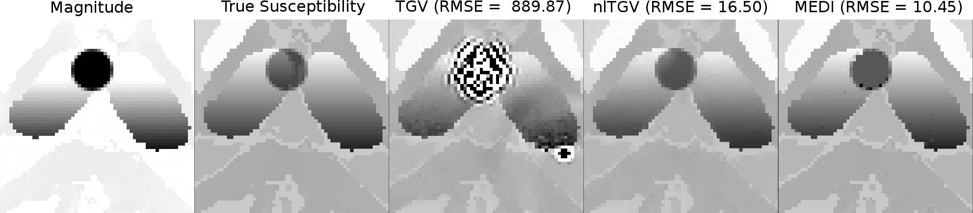
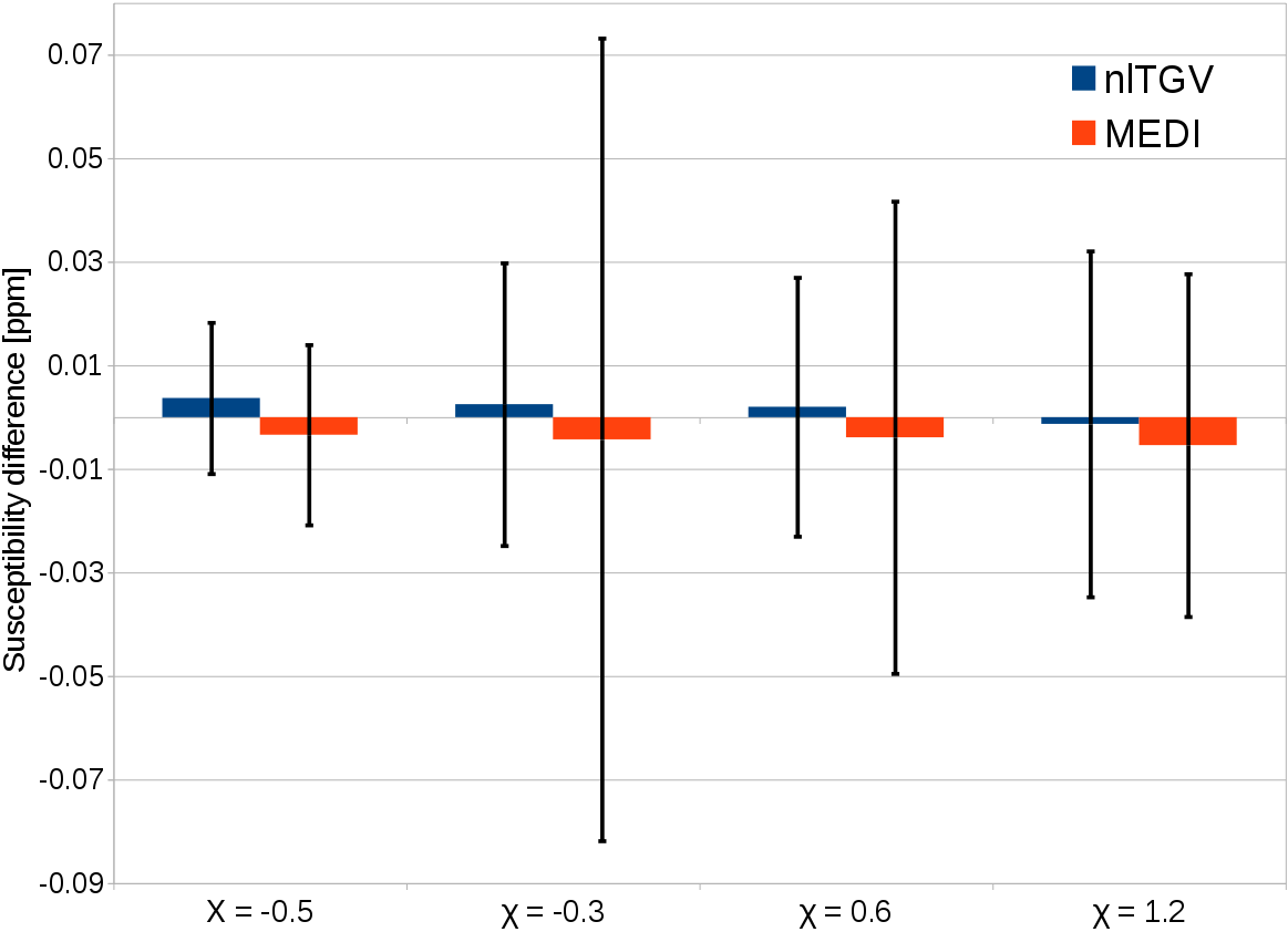
A) Synthetic brain phantom with 4 simulated "lesions". Each lesion was a sphere of constant susceptibility (-0.3ppm, -0.5ppm, 0.6ppm and 1.2ppm, respectively) and zero magnitude. Results were evaluated by mean error and std-dev at each sphere and global RMSE.
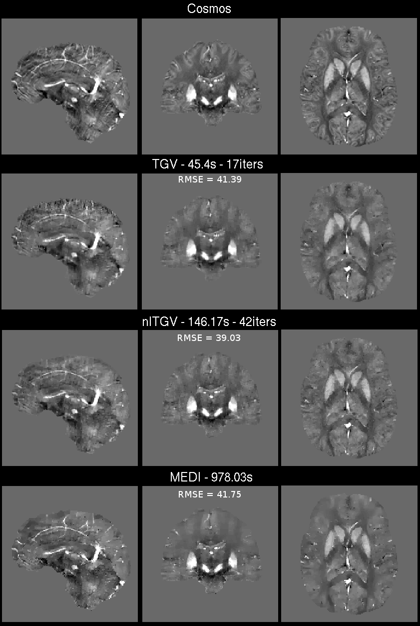
B) COSMOS [9] reconstruction (3D-GRE with Wave-CAIPI at 3T Siemens Tim Trio, 1.06×1.06×1.06 mm3 isotropic, 240×196×120, TE/TR = 25/35 ms, 12 orientations) was used as susceptibility ground truth, from which the starting field map was forward-simulated. The magnitude from a single acquisition was also used, normalized from 0 to 1, to create complex data in the image domain. Gaussian noise was added with an amplitude of 2% (SNR = 50). The noise-corrupted phase was used as input for the algorithms.
C) 3T MRI in vivo data (Siemens Tim Trio, 32 channel head array, 1 mm3 isotropic resolution, 240×192×120 mtx, TE/TR = 24.8/35 ms, Tacq=13.5min). Phase unwrapping and background subtraction were performed with Laplacian [10] and Laplacian Boundary Value (LBV) [11] methods, respectively. Results were evaluated qualitatively in terms of artifact reduction and noise management.
RESULTS
A) Global RMSE scores and details for one of the lesions are shown in Fig. 1. Mean susceptibility errors and standard deviation for each lesion are shown in Fig. 2.
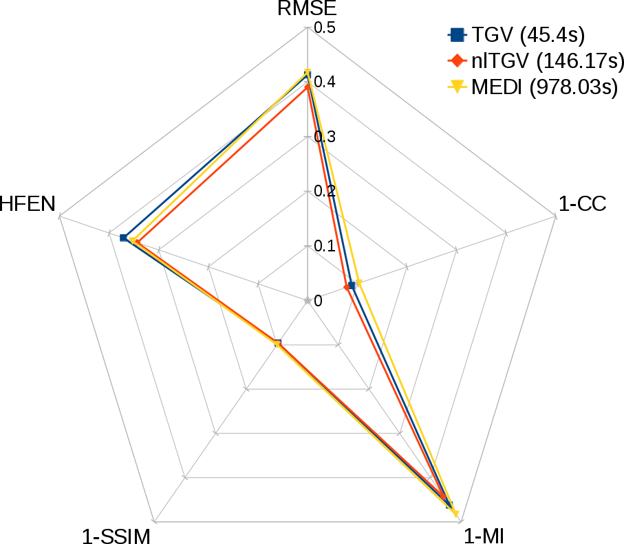
B) Fig. 3 shows the reconstruction results. Fig. 4 shows the normalized scores for each quality metric (RMSE, High Frequency Error Normalized, Structural Similitude, Mutual Information and Correlation Coefficient) and time.
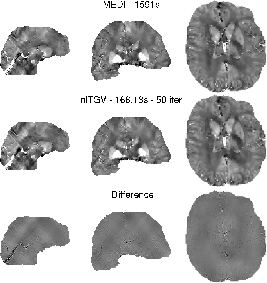
C) Fig. 5 shows the results with nlTGV and MEDI, along with a difference map.
DISCUSSION
The above results confirmed an improvement for the proposed formulation over linear TGV in terms of noise management and in preventing streaking artifacts emanating from zero or low SNR regions. Compared to nonlinear MEDI, nlTGV yielded similar reconstructions, yet with a small systematic advantage in quality metrics and accuracy. Differences can be explained by the type of regularization employed; whilst MEDI promotes piece-wise constant QSM reconstructions aided by edge information in magnitude data, nlTGV promotes piece-wise smooth solutions. The latter prior appears to be better suited for in vivo data, as it reduces QSM’s ‘cartoonish’ appearance. Nevertheless, incorporating prior knowledge from magnitude data would help the proposed formulation to protect small-scale features. The major difference between the two approaches was computational time; notably, nlTGV was 6,7 to 9,6 times faster than MEDI.CONCLUSION
Our proposed algorithm provides a substantial gain in computational efficiency compared to MEDI, with marginal—albeit systematic— quality performance gain in phantom experiments.Acknowledgements
The authors gratefully acknowledge support from FONDECYT 1161448 and ANILLO ACT1416 Programa PIA CONICYT. CM thanks CONICYT and Ministry of Education of Chile, with his higher education program, for scholarship for doctoral studies.References
1. Gudbjartsson H, Patz S. The Rician distribution of noisy MRI data. Magnetic Resonance in Medicine. 1995;34(6):910–914.
2. Liu T, Wisnieff C, Lou M, Chen W, Spincemaille P, Wang Y. Nonlinear formulation of the magnetic field to source relationship for robust quantitative susceptibility mapping. Magnetic resonance in medicine : official journal of the Society of Magnetic Resonance in Medicine / Society of Magnetic Resonance in Medicine. 2013;69(2):467–76.
3. Wang S, Liu T, Chen W, Spincemaille P, Wisnieff C, Tsiouris a J, Zhu W, Pan C, Zhao L, Wang Y. Noise Effects in Various Quantitative Susceptibility Mapping Methods. Biomedical Engineering, IEEE Transactions on. 2013;60(12):3441–3448.
4. Yanez F, Fan A, Bilgic B, Milovic C, Adalsteinsson E, Irarrazaval P. Quantitative Susceptibility Map Reconstruction via a Total Generalized Variation Regularization. 2013 International Workshop on Pattern Recognition in Neuroimaging. 2013 Jun:203–206
5. Langkammer C, Bredies K, Poser B a., Barth M, Reishofer G, Fan AP, Bilgic B, Fazekas F, Mainero C, Ropele S. Fast quantitative susceptibility mapping using 3D EPI and total generalized variation. NeuroImage. 2015;(2014).
6. Bilgic B., Chatnuntawech I., Langkammer C., Setsompop K.; Sparse Methods for Quantitative Susceptibility Mapping; Wavelets and Sparsity XVI, SPIE 2015
7. Ramani S, and Fessler J. A. , Parallel MR Image Reconstruction Using Augmented Lagrangian Methods, in IEEE Transactions on Medical Imaging, vol. 30, no. 3, pp. 694-706, March 2011.
8. Zhao B, Lam F., Bilgic B., Ye H. and Setsompop K., Maximum likelihood reconstruction for magnetic resonance fingerprinting, 2015 IEEE 12th International Symposium on Biomedical Imaging (ISBI), New York, NY, 2015, pp. 905-909. 9. Liu T, Spincemaille P, De Rochefort L, Kressler B, Wang Y. Calculation of susceptibility through multiple orientation sampling (COSMOS): A method for conditioning the inverse problem from measured magnetic field map to susceptibility source image in MRI. Magnetic Resonance in Medicine. 2009;61(1):196–204. 10. Li W, Wu B, Liu C. Quantitative susceptibility mapping of human brain reflects spatial variation in tissue composition. NeuroImage. 2011;55(4):1645–1656. 11. Zhou D, Liu T, Spincemaille P, Wang Y. Background field removal by solving the Laplacian boundary value problem. NMR in Biomedicine. 2014;27(3):312–319.
Figures