3667
Accelerated $$$B_{0}$$$ Mapping Using "X" Sampling in $$$k$$$-TE Space1Biomedical Engineering, University of Southern California, Los Angeles, CA, United States, 2Ming Hsieh Department of Electrical Engineering, University of Southern California, Los Angeles, CA, United States, 3Division of Cardiology, Children's Hospital Los Angeles, Los Angeles, CA, United States
Synopsis
High-resolution B0 mapping suffers from long scan time, and issues with phase-wraps. We present an acquisition and reconstruction technique that resolves both problems. We utilize “X” sampling in k-TE space, in which multiple phase-encoding lines are acquired exactly twice per TR. The echo spacing is shortest for central k-space and largest for outer k-space. A multi-scale reconstruction enables pixel-wise phase unwrapping. This technique may be particularly useful for quantitative susceptibility mapping (QSM), as it could a) shorten scan time while maintaining the sensitivity to high-order field variation and b) simplify phase-unwrapping, which are the key features of interest in QSM.
Purpose
High-resolution B0 mapping is critical to quantitative susceptibility mapping (QSM). Long echo times (TE = 20-40 ms) are needed to optimize the sensitivity to high-order field variation and tissue susceptibility1-3. However, this causes long scan time and phase-wraps. In this study, we propose a new approach that utilizes “X”-pattern sampling in $$$k$$$-TE space, where echo spacing varies with $$$k$$$-space position. The corresponding reconstruction combines multi-scale estimation and non-linear optimization. The aim is to a) shorten scan time while maintaining the sensitivity to high-order field variation and b) simplify phase-unwrapping.Theory
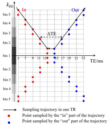
Figure 1 shows the proposed sampling scheme. Positive and negative halves of $$$k$$$-space are divided into $$$N$$$ bins. In each TR, $$$N$$$ phase-encoding (PE) lines are acquired, each exactly twice. The echo time difference (ΔTE) increases with the magnitude of $$$k_{PE}$$$.
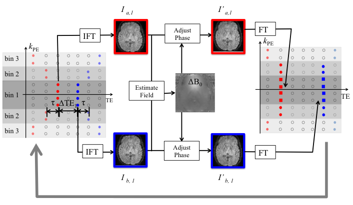
Field estimation is performed at multiple spatial scales. The first (coarsest) scale corresponds to the central k-space bin, which has the shortest ΔTE. Figure 2 shows the first iteration. Step 1: Bin 1 is extracted and the other regions are zero-filled. The early-TE (red dots) and late-TE (blue dots) samples are inverse Fourier transformed to $$$I_{a,1}$$$ and $$$I_{b,1}$$$. Step 2: $$$\Delta B_{0}^{1}$$$ is estimated: $$$\Delta B_{0}^{1} = \frac{\angle (I_{a,1}\cdot I_{b,1}^{*})}{\gamma 2\pi \Delta TE_{1}}$$$. Note that $$$\Delta B_{0}^{1}$$$ is free of wraps when $$$\Delta TE_{1}$$$ is smaller than the reciprocal of the resonant frequency range. Step 3: The phase of $$$I_{a,1}$$$ and $$$I_{b,1}$$$ are adjusted using $$$\Delta B_{0}^{1}$$$ to match the echo times of bin 2: $$$I_{a,1}^{'} = I_{a,1}\cdot e^{+j\gamma 2\pi \Delta B_{0}^{1}\tau }$$$, $$$I_{b,1}^{'} = I_{b,1}\cdot e^{-j\gamma 2\pi \Delta B_{0}^{1}\tau }$$$ Step 4: Bin 1 is updated by the Fourier transform of $$$I_{a,1}^{'}$$$ and $$$I_{b,1}^{'}$$$ (red and blue squares). Bin 1 and bin 2, now with the same effective echo times, are combined for the next iteration. In the $$$i$$$th iteration, when $$$\Delta B_0^{i}-\Delta B_0^{i-1}$$$ is less than the reciprocal of $$$\Delta TE_i$$$, pixel-by-pixel phase-unwrapping can be performed perfectly using $$$\Delta B_0^{i-1}$$$ as a reference. After $$$N$$$ iterations, $$$\Delta B_{0}^{N}$$$ is the result of multi-scale estimation. As a final step, a non-linear optimization is performed using $$$\Delta B_{0}^{N}$$$ as the initial guess: $$\Delta B_{0}^{nonlin}\left ( \boldsymbol{r} \right )=\arg min_{\Delta B_0 \left ( \boldsymbol{r} \right )} \left \| \mathcal{F}_u \{\hat{M}\left ( \boldsymbol{r} \right ) e^{-j\left ( \hat{\psi _0}\left ( \boldsymbol{r} \right )+\gamma 2\pi \Delta B_0 \left ( \boldsymbol{r} \right )TE \right ) } \}-S\left ( \boldsymbol{k},TE \right )\right \|_2^2$$, where $$$\mathcal{F}_u$$$ represents the “X”-pattern Fourier under-sampling in $$$k$$$-TE space, $$$\hat{M}\left ( \boldsymbol{r} \right )$$$ is the estimated magnitude image, $$$\hat{\psi _0}\left ( \boldsymbol{r} \right )$$$ is the phase at TE = 0 estimated from the central $$$k$$$-space bin, $$$S\left ( \boldsymbol{k},TE \right )$$$ is multi-echo $$$k$$$-space data.
Methods
Data: 3D Multi-echo GRE data were synthesized using:$$m\left ( \boldsymbol{r},TE \right )=\rho \left ( \boldsymbol{r} \right ) e^{-TE/T_2^{*}\left ( \boldsymbol{r} \right )} e^{-j\left ( \psi _0 \left ( \boldsymbol{r} \right )+\gamma 2\pi \Delta B_0 \left ( \boldsymbol{r} \right )TE \right )}+n\left (\boldsymbol{ r},TE \right )$$, where proton density $$$\rho \left ( \boldsymbol{r} \right )$$$, $$$T_2^{*}$$$ map $$$T_2^{*}\left ( \boldsymbol{r} \right )$$$, low-resolution phase offset $$$\psi _0 \left ( \boldsymbol{r} \right )$$$, and field map $$$\Delta B_0 \left ( \boldsymbol{r} \right )$$$ were taken from a fully-sampled multi-echo GRE scan of a healthy volunteer. Acquisition parameters: 3 Tesla GE Signa HD23, spatial resolution = 0.5 mm (AP) x 0.5 mm (RL) x 1 mm (SI), TE = 5,10,15,20 ms, TR = 50 ms, BW = ±62.5kHz. $$$n\left ( r,TE \right )$$$ was i.i.d. bivariate gaussian noise scaled to make the white matter SNR equal 40. Simulated acquisition: We simulated a 5-bin acquisition ($$$N=5$$$, divided along $$$k_y$$$), and ten echo times: 5,7,9,11,13,15,17,19,21,23 ms. The $$$k_z$$$ phase-encoding direction was fully-sampled. Evaluation: Projection onto dipole field (PDF)4,5 was used to extract the high-order field variation originating from tissue susceptibility difference (“local field”). Both the total $$$\Delta B_0$$$ and the "local field" of the estimation were evaluated.
Results & Discussion
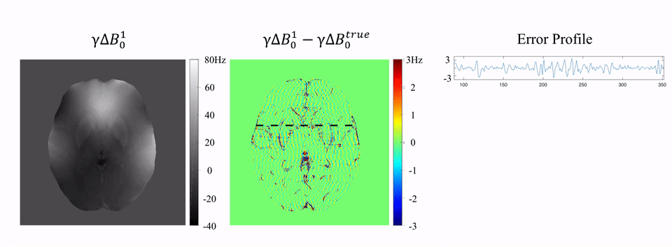
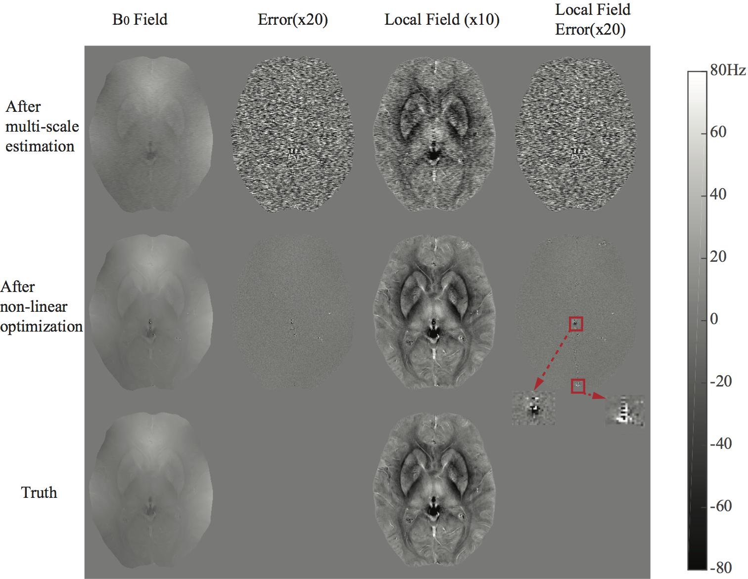
Figure 3 shows multi-scale estimation in a noiseless case. Fine structures were iteratively revealed in the reconstruction. Figure 4 shows the case with noise. Non-linear optimization has less error, indicating more noise-resistance than multi-scale estimation alone. In the "local field" evaluation, non-linear optimization reliably reconstructed the field around tissue structures (e.g. basal ganglia nuclei). Poor depiction of the field near through-plane veins (red arrows) was observed. This may affect susceptibility quantification near these veins.Conclusion
This study demonstrates a new accelerated approach to high-resolution B0 mapping, which utilizes “X” sampling in k-TE space and a novel reconstruction. The proposed method, as simulated, potentially shortens scan time by 5-fold compared to conventional multi-echo sequences1,3 and enables pixel-wise phase-unwrapping. Prospective application of this approach to in-vivo QSM remains as future work.Acknowledgements
This work is supported by the National Heart Lung and Blood Institute (1U01HL117718-01).References
1. Haacke EM, et al. Quantitative susceptibility mapping: current status and future directions. Magnetic resonance imaging. 2015 Jan 31;33(1):1-25.
2. Haacke EM, Brown RW, Thompson MR, Venkatesan R. Magnetic resonance imaging: physical principles and sequence design. 1st ed. Wiley-Liss; 1999.
3. Wang Y, Liu T. Quantitative susceptibility mapping (QSM): decoding MRI data for a tissue magnetic biomarker. Magnetic resonance in medicine. 2015 Jan 1;73(1):82-101.
4. Liu, T, et al. A novel background field removal method for MRI using projection onto dipole fields (PDF). NMR in Biomedicine 24.9 (2011): 1129-1136.
5. de Rochefort L, et al. Quantitative susceptibility map reconstruction from MR phase data using bayesian regularization: validation and application to brain imaging. Magnetic resonance in medicine. 2010 Jan 1;63(1):194-206.
Figures