3660

Magnetic Properties of Skeletal Muscle at 7T

Benjamin Tendler¹ and Richard Bowtell¹

¹Sir Peter Mansfield Imaging Centre, University of Nottingham, Nottingham, United Kingdom

Synopsis

The magnetic properties of skeletal muscle tissue were examined in a phantom consisting of a piece of muscle tissue embedded in agar. Frequency perturbation maps were generated from phase maps measured at 7T, with the phantom oriented at 29 angles to the external magnetic field. Using a novel minimisation technique, susceptibility and chemical exchange properties of the muscle tissue were obtained simultaneously. From this it was determined that skeletal muscle is significantly more diamagnetic than agar; there is a small anisotropic susceptibility component and a large, orientation independent positive offset within the tissue, hypothesised to be due to chemical exchange.

Introduction

There has been longstanding interest in the magnetic properties of muscle tissue,¹ but to date there has been little examination of these properties using MRI-based measurements of frequency perturbations. Such measurements could provide a valuable way of probing the structure and function of muscle tissue, revealing information about its microstructure, magnetic properties and molecular composition. Here we describe an examination of magnetic properties based on frequency mapping measurements carried out at 7T on phantoms containing a small piece of muscle (pork tenderloin) embedded in agar, measuring the susceptibility tensor, $$$\chi$$$, and the chemical exchange, $$$E$$$, properties of the tissue.

Theory

Previous research has commonly employed isotropic susceptibility, $$$\chi_{I}$$$, as a means to explain the contrast provided by frequency perturbations in phase images. However, recent work has indicated that isotropic susceptibility is not always sufficient to explain the measured frequency perturbations. One method of further describing the frequency perturbations involves removing the assumption that susceptibility is isotropic and describing susceptibility by a generalised 3x3 symmetric susceptibility tensor,² $$$\chi$$$. In addition, the chemical exchange, $$$E$$$, properties of tissue have been described by an orientation independent, local offset.^3-4 Here a novel minimisation technique was developed, based on the MMSR-STI method,⁵ but with an additional term describing chemical exchange. The following minimisation was applied to frequency maps acquired with the sample oriented at multiple angles to the static field, $$$B_{0}$$$:

$$min_{\chi,E}\Bigg(\left\| W_{0}\left(\Delta B-B_{0}F^{-1}\left[F\left[\chi\right]\cdot F\left[D\right]\right]-\frac{2\pi E}{\gamma}\right)\right\|_{2}^{2}+\sum_{i=1}^{3}\sum_{j=i+1}^{3}\beta_{1}^{2}\left(\left\|W_{1}\chi_{ij}\right\|_{2}^{2}+ \left\|W_{1}\left(\chi_{ii}-\chi_{jj}\right)\right\|_{2}^{2}\right)+\beta_{2}^{2}\left\|W_{2}E\right\|_{2}^{2}\Bigg)$$

where $$$W_{0}$$$ is the magnitude image, $$$\Delta B$$$ are the measured frequency perturbations, $$$F$$$ and $$$F^{-1}$$$ are the Fourier & inverse Fourier transforms, $$$D$$$ is the dipole field,² $$$\gamma$$$ is the gyromagnetic ratio, $$$W_{1}$$$ is an isotropic weighting mask, $$$W_{2}$$$ is the exchange weighting mask and $$$\beta_{1}$$$ and $$$\beta_{2}$$$ are regularisation coefficients.

Method

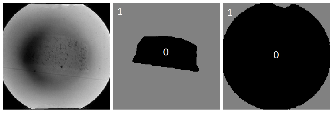
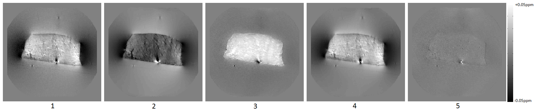
A sample of pork-tenderloin was trimmed and stripped of external fat prior to being embedded in agar (1.2% agar, 0.9% NaCl). Using a Philips Achieva 7T MR scanner, the sample underwent a series of dual echo GE scans (resolution =1mm³, 160x160x160mm³, TE₁=8ms and TE₂=20ms, TR=21.6ms, flip angle=15^o, acquisition time=553s). The sample was scanned at 29 angles with respect to the static field. Phase was processed via the complex division of the two phase echoes, followed by phase unwrapping using the Hussein, path-based unwrapping algorithm,⁶ and filtering using v-SHARP with high-pass regularisation of 0.005mm,⁷ and a maximum spherical radius of 8mm. Images were coregistered manually using the mrAlign toolbox.⁸ Using the equation outlined above, an LSQR fitting algorithm was implemented to determine $$$\chi$$$ and $$$E$$$ simultaneously. $$$\beta_{1}$$$ and $$$\beta_{2}$$$ were both set to 10⁸ to force the regularisation conditions. $$$W_{1}$$$ was defined to force isotropy in regions surrounding the muscle tissue .$$$W_{2}$$$ was defined as the mask external to the agar and muscle tissue, to prevent fitting of chemical exchange to the regions outside the phantom. $$$W_{0}$$$, $$$W_{1}$$$ and $$$W_{2}$$$ are displayed in Figure 1.

Results

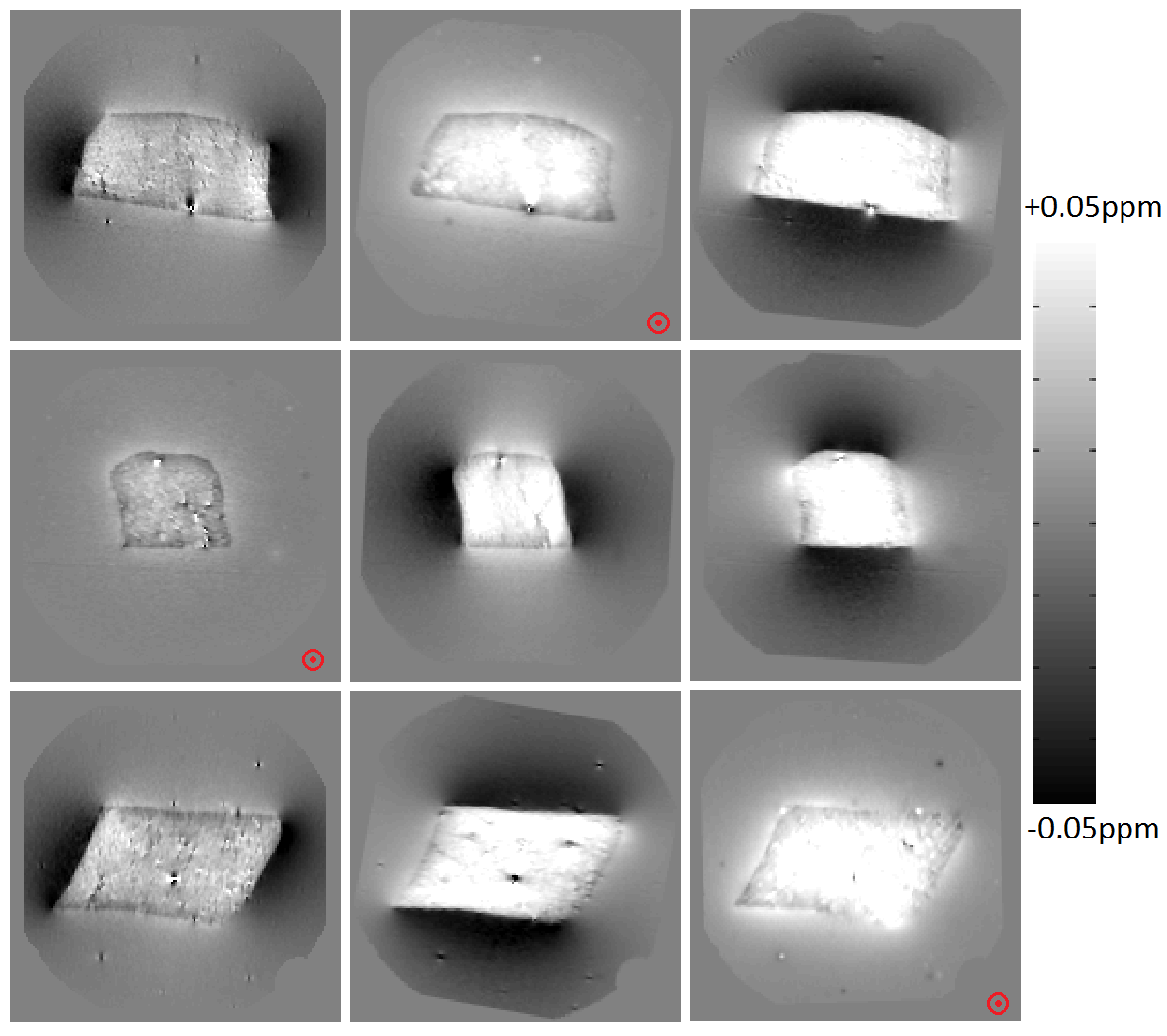
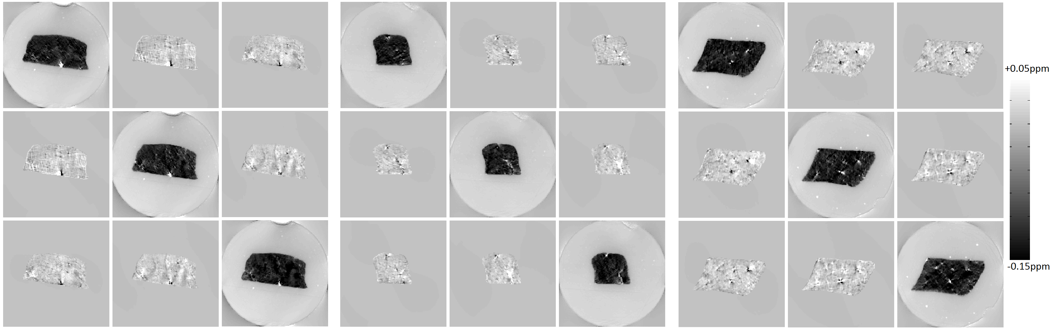
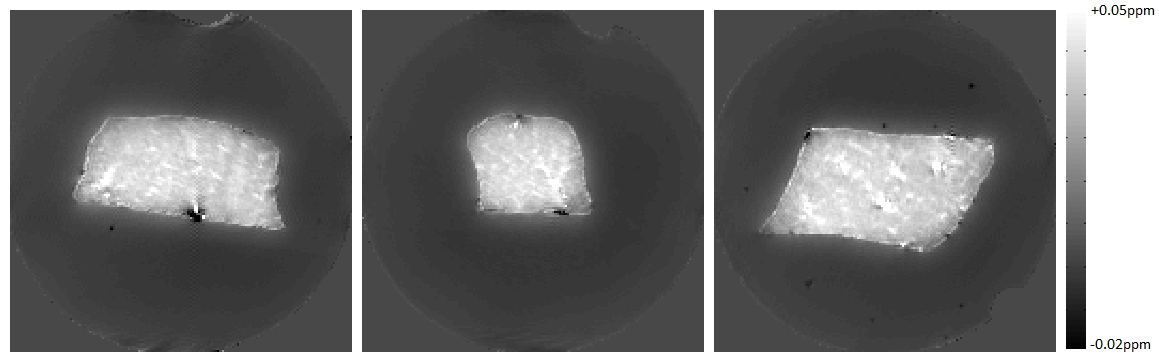
Examples of the measured frequency perturbation maps are shown in Figure 2. The susceptibility tensor, $$$\chi$$$ and chemical exchange, $$$E$$$, maps obtained from the minimisation are shown in Figures 3 & 4. A comparison of measured and simulated frequency perturbations is displayed in Figure 5.

Discussion

The experimental work has indicated that isotropic susceptibility is not sufficient to explain the frequency perturbations within muscle tissue and an additional chemical exchange component is necessary to describe the contrast within the muscle tissue phantom. Subtraction of the simulated frequency perturbations from the measured frequency perturbations in Figure 5 yields a residual that shows significant contrast only in areas containing air bubbles within the phantom when contributions from both susceptibility and chemical exchange are considered. When only susceptibility contributions are considered, significant contrast remains throughout the entire skeletal muscle sample when examining the residual.

Analysis of Figure 3 reveals that muscle tissue is significantly more diamagnetic that the surrounding agar, with mean isotropic susceptibility values of $$$\chi_{I:muscle}$$$=(-0.11$$$\pm$$$0.02)ppm and $$$\chi_{I:agar}$$$=(0.01$$$\pm$$$0.01)ppm, where $$$\pm$$$ indicates the standard deviation. There is additionally evidence of a small anisotropic susceptibility component. Furthermore, the $$$E$$$ map (Figure 4) indicates that there is significant chemical exchange within the muscle tissue that does not occur within the surrounding agar, with $$$E_{muscle}$$$=(0.03$$$\pm$$$0.01)ppm and $$$E_{agar}$$$=(-0.003$$$\pm$$$0.003ppm). In addition to the residual, artefacts are noted within the $$$\chi$$$ and $$$E$$$ maps surrounding the air bubbles and blood vessels within the tissue. Further work is needed to investigate the origin of the chemical exchange and to characterise the anisotropy in relation to the orientation of muscle fibres, to prepare for in-vivo characterisation of muscle tissue.

Acknowledgements

No acknowledgement found.

References

1.Arnold, W., R. Steele, and H. Mueller., Proceedings of the National Academy of Sciences of the United States of America, 1958

2.Liu C., Magnetic Resonance in Medicine, 63(6):1471–7, 2010.

3.Shmueli, K., et al., J. H., Magnetic resonance in Medicine 65: 35–43, 2011

4.Wharton, S. and Bowtell, R., Magnetic Resonance in Medicine, 73: 1258–1269, 2015

5.Li X. and van Zijl PC., Magnetic Resonance in Medicine, 72(3): 610–619, 2014

6.Abdul-Rahman HS., et al., Applied Optics, 46(26): 6623–35, 2007

7.Özbay. P et al, NMR in Biomedicine, 2016

8.Nestares, Oscar. and David J. Heeger., Magnetic Resonance in Medicine, 43(5): 705-715, 2000

Figures

Figure 1: Weighting masks used for fitting. $$$W_{0}$$$ (left) corresponds to magnitude data, $$$W_{1}$$$ (middle) corresponds to the mask external to muscle tissue and $$$W_{2}$$$ (right) corresponds to the mask external to muscle tissue and agar. Masks are shown in a single central plane

Measured frequency perturbations for three separate orientations of the muscle tissue with respect to the magnetic field (left to right) and three orthogonal planes through the centre of the sample (top to bottom). Direction of external magnetic field highlighted in red.

Figure 3: 3x3 susceptibility tensor, $$$\chi$$$, of the muscle tissue and agar, for 3 orthogonal planes through the centre of the sample (left to right), determined from fitting to the experimental data. Units in parts per million.

Figure 4: Chemical exchange component, $$$E$$$, of the muscle tissue and agar, for 3 orthogonal planes through the centre of the sample (left to right) determined from fitting to the experimental data. Units in parts per million.

Figure 5: From left to right: 1. Measured frequency perturbations for a single slice, single orientation scan through the centre of the sample. 2. Simulated frequency perturbations for susceptibility component. 3. Remaining residual from subtracting frequency perturbations of susceptibility component from experimental data. 4. Simulated frequency perturbations for susceptibility and exchange component. 5 Remaining residual from subtracting frequency perturbation of susceptibility and exchange components from experimental data. Units in parts per million.

Proc. Intl. Soc. Mag. Reson. Med. 25 (2017)

3660