3652
Quantitative susceptibility mapping with separate calculation in water and fat regions1Research and Development Group, Hitachi, Ltd., Tokyo, Japan, 2Healthcare Business Unit, Hitachi, Ltd., Tokyo, Japan
Synopsis
To reduce the calculation error and artifacts of susceptibility in the boundary region between water and fat, a new reconstruction method is presented and applied to a prostate QSM. In the proposed method, susceptibility maps of the water region and the fat region are calculated separately and differently and then combined. Numerical simulation and human prostate imaging using a 3T-MRI are performed to evaluate accuracy and artifacts of the proposed method. The results suggest that the proposed method reduces calculation error and the shading artifacts in the boundary region between water and fat near the prostate.
Purpose
Quantitative susceptibility mapping (QSM) is expected to be used in the diagnosis of diseases affecting different areas of the body1-3, such as iron overload in the liver2 and prostate cancer3. The presence of fat in different body areas sometimes causes calculation errors in the boundary region between water and fat because of signal loss in bones or air near the fat regions. This error results in shading artifacts of susceptibility and may reduce the accuracy in areas to be diagnosed such as the prostate adjacent to subcutaneous fat. To reduce the calculation error and artifacts, we have developed a method to calculate the susceptibilities in water and fat regions separately and evaluated it by numerical simulation and several volunteers’ study in a prostate QSM.
Methods
Proposed method: A susceptibility map of the water region $$$\chi_w$$$ and a susceptibility map of the fat region $$$\chi_f$$$ are calculated separately from a frequency map $$$f_0$$$ obtained using the multi-point Dixon method, and then combined. The water region $$$M_w$$$ and fat region $$$M_f$$$ are defined by thresholding a fat fraction map. The process flow is shown in Fig. 1. First, in the calculation of $$$\chi_w$$$, background-removed frequency map in water $$$f_w$$$ is calculated with the fat region regarded as a background susceptibility source to remove artifacts caused by susceptibility differences between the water and fat. Then,$$$\chi_w$$$ is calculated from $$$f_w$$$4. Second, in the calculation of $$$\chi_f$$$, the background-removed frequency map in water and fat $$$f_{f+w}$$$ is calculated, and then $$$\chi_f$$$ is calculated from $$$f_{f+w}$$$ with the constraint that the susceptibility in the water region $$$M_w$$$ is zero in accordance with the following equation, $$\chi_f = argmin _{\chi_f} ||(M_w+M_f) (Cχ_f-δ)||_2^2 + λ_w||M_wχ_f||_2^2 + λ_f||M_fGχ_f||_2^2,$$ where $$$C$$$ denotes a matrix representing convolution of the dipole kernel, $$$\delta$$$ denotes a local field calculated from $$$f_{f+w}$$$, $$$G$$$ denotes the three-dimensional gradient operator, and $$$\lambda_w$$$ and $$$\lambda_f$$$ denote regularization parameters. By using the second term in the above equation, $$$\chi_f$$$ can be calculated under condition in which shading artifacts do not occur in the water region. Finally, the susceptibility map $$$\chi$$$ is calculated by combining $$$\chi_w$$$ and $$$\chi_f$$$.
Numerical simulation: Numerical simulation was used to compare the accuracy of the conventional4 and proposed methods. The susceptibility model (Fig. 2(a)) with water and fat regions was designed using a fat fraction map obtained in a human volunteer experiment. The frequency map was calculated from this model using a forward method5 (B0: 3 T) with Gaussian noise added to each voxel (SD: 1.5 Hz). Then, susceptibility maps were calculated by the conventional and proposed methods.
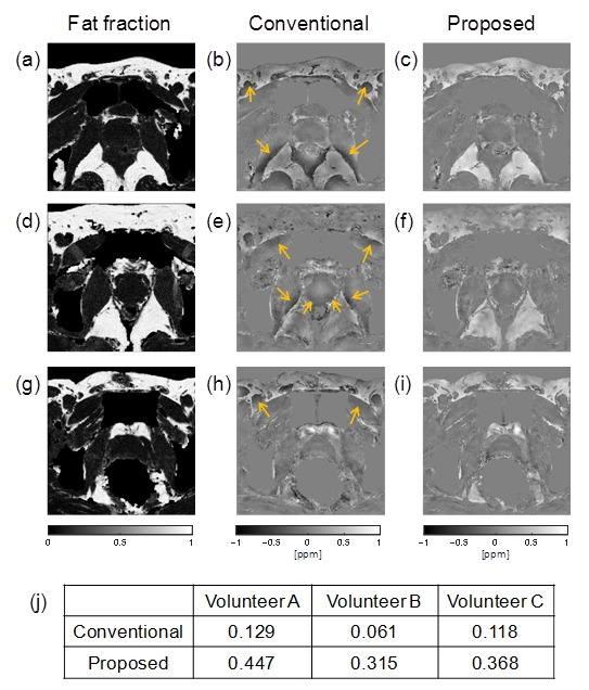
Human volunteer experiment: To compare the shading artifacts and susceptibilities of the conventional4 and proposed methods, three healthy volunteers were scanned using 3D RF spoiled gradient echo in a 3T MRI (Hitachi, Ltd. Japan). The main parameters for all scans are as follows: TR: 45ms; TE: 7.0/ 10.5/ 14.0/ 17.5/ 21.0/ 24.5ms; matrix: 208×192×20 (reconstructed to 512×512×20); and FOV: 160×160×66mm. Data of the volunteers were obtained in accordance with the regulations of the internal review board of the Central Research Laboratory, Hitachi, Ltd., following receipt of informed consent.
Results and discussion
In the numerical simulation, shading artifacts around fat regions in the susceptibility map calculated by the conventional method occurred (shown with arrows in Fig. 2(b)), whereas no artifacts occurred in the susceptibility map calculated by the proposed method (Fig. 2(c)). The RMSE between the model and the susceptibility in the fat region was lower for the proposed method (0.05 ppm) than for the conventional method (0.33 ppm). This result suggests that the accuracy of the susceptibility in the fat region improves with the accuracy of the susceptibility in the region around the fat under the constraint that shading artifacts do not occur in the water region.
In the human volunteer experiment, as shown in Figs.3(a)-(i), shading artifacts around fat regions were reduced by the proposed method. As shown in Fig.3(j), the mean susceptibilities of the fat region (referenced to internal obturator muscle) calculated by the proposed method were closer to the standard value of susceptibility difference between water and fat (0.61 ppm6) than those obtained by the conventional method in all three cases. Mean value in three volunteers is 17% of the standard value in the conventional method, and 62% in the proposed method. These results suggest that the accuracy in the fat region improves by the proposed method in human volunteer experiment.
Conclusion
The proposed method reduces the shading artifacts and calculation error in the boundary region between water and fat near the prostate.Acknowledgements
No acknowledgement found.References
1. Dimov AV, Liu T, Spincemaille P, et al. Joint estimation of chemical shift and quantitative susceptibility mapping (chemical QSM). Magn Reson Med. 2015; 73: 2100-2110.
2. Sharma SD, Hernando D, Horng DE, Reeder SB. Quantitative susceptibility mapping in the abdomen as an imaging biomarker of hepatic iron overload. Magn Reson Med. 2015; 74: 673-683.
3. Straub S, Laun FB, Emmerich J, et al. Potential of quantitative susceptibility mapping for detection of prostatic calcifications. J Magn Reson Imaging. 2016; in press.
4. Sato R, Shirai T, Taniguchi Y, Murase T, Bito Y, Ochi H. Improving estimation of small-vein susceptibility by using a pre-estimated susceptibility map. Proc Intl Soc Mag Reson Med. 2015; 23: 927.
5. Marques JP and Bowtell R. Application of a Fourier-based method for rapid calculation of field inhomogeneity due to spatial variation of magnetic susceptibility. Concepts Magn Reson. Part B. 2005; 25: 65-78.
6. Szczepaniak LS, Dobbins RL, Stein DT, McGarry JD. Bulk magnetic susceptibility effects on the assessment of intra- and extramyocellular lipids in vivo. Magn Reson Med. 2002; 47: 607-610.
Figures
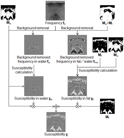
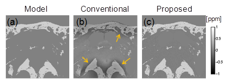
Fig. 2 Results of numerical simulation. (a) Model susceptibility. (b)(c) Susceptibility maps calculated with conventional and proposed methods. Shading artifacts are shown by arrows.