3643
Adaptive Weighted Polynomial fitting in phase-based Electrical Property Tomography1Department of Electrical and Electronic Engineering, Yonsei University, seoul, Korea, Republic of, 2Department of Radiology and Research Institute of Radiological Science, Severance Hospital, Yonsei University College of Medicine, seoul, Korea, Republic of
Synopsis
Weighted polynomial fitting method was proposed to resolve boundary artifact and noise amplification of Electrical Property Tomography. Weighted polynomial fitting method employs T1/T2 tissue contrast as prior information under assumption that pixels with similar magnitude intensity have similar conductivity. However, for non-simply connected structures make the fitting inaccurate. Therefore, in this study, we propose a modified weighted polynomial fitting technique including spatial constraint.
Introduction
Electrical Property Tomography(EPT) has two inherent problems in the reconstruction process: boundary artifact and noise amplification [1]. Recently, several research has proposed reconstruction algorithms to resolve these two problems including gradient-based EPT [2], inverse method [3], and weighted polynomial fitting [4]. Among them, the weighted polynomial fitting method employs T1/T2 tissue contrast as prior information under assumption that pixels with similar magnitude intensity have similar conductivity. However, for non-simply connected structures such as seen in the cortex, nearby pixels have different T1/T2 signal intensity make the fitting inaccurate. In this study, we propose an adaptive weighted polynomial fitting technique which include spatial constraints. For verification, this technique was evaluated using a simulation phantom. In addition, this technique was applied in-vivoTheory & Implementation
In previous studies employing the weighting fitting scheme, the weights were determined using only tissue contrast (Eq.1).
$$$W_{m} (r) = \frac{1}{\sigma_ {mag}\sqrt{2\pi}} e^{-(\mid I(r)-I(r_0) \mid)/2(\sigma_{mag})^2)}$$$ (Eq.1)
where I(x,y) is intensity of prior image, $$$\sigma_{mag}$$$ is standard deviation of magnitude weighting function and $$$x_0, y_0$$$ are the center of kernel.
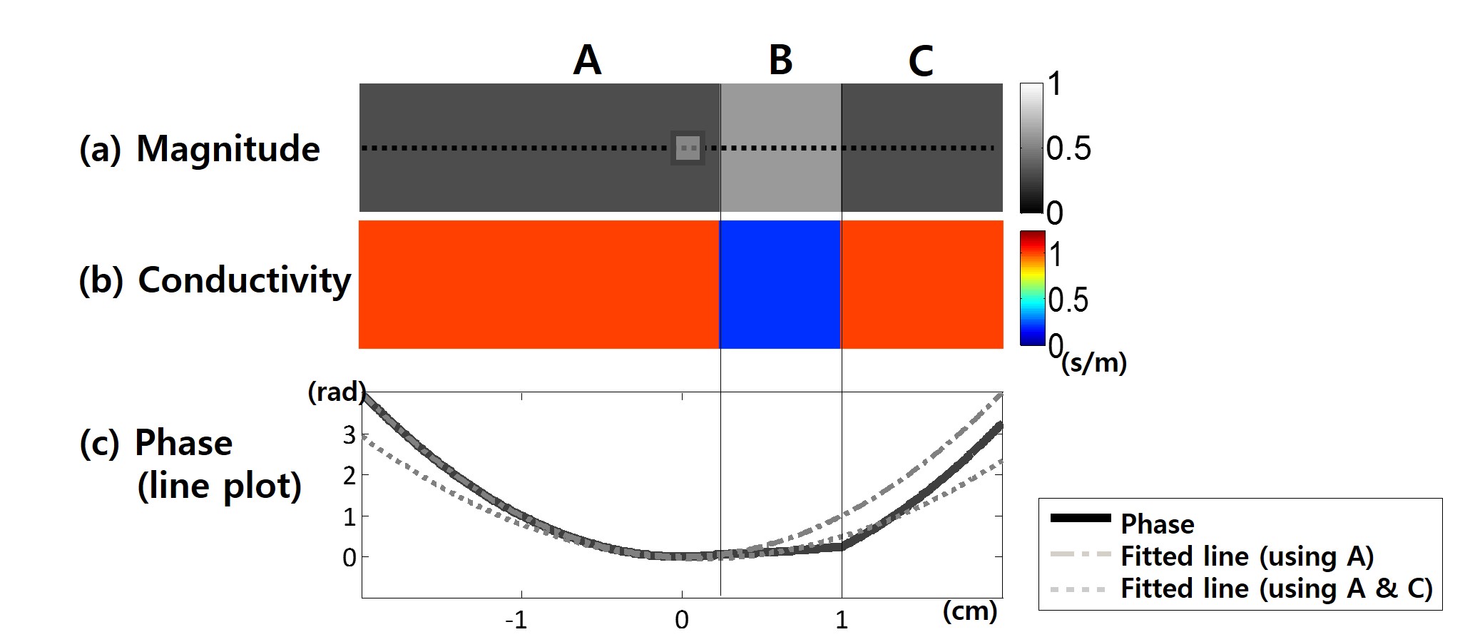
In Figure 1, a 1-dimensional example is presented to demonstrate the limitation of fitting for non-simply connected regions. Over the region with same conductivity (region A&C), $$$B_1$$$ phase is propagated with the same curvature as shown in Fig.1c. However, in spite of the same conductivity value in these two regions, there is zeroth-order offset due to the presence of region B with different conductivity. For the case of fitting over the regions A&C, this offset hampers estimation of the curvature as shown by the dotted line in Fig.1c. Therefore, an additional spatial constraint is necessary to extract the local conductivity value. At first, spatial constraint was designed as isotropic-gaussian function (FWHM=1/4 of kernel size) as Eq.2 and (Eq.1) was combined.
$$$W_{S1} (r) = \frac{1}{\sigma_ {S}\sqrt{2\pi}} e^{-(\mid I(r)-I(r_0) \mid)/2(\sigma_{S})^2}$$$ (Eq.2)
where $$$ \sigma_S$$$ is standard deviation of spatial weighting function.
In addition, to take into account structures such as the cortex regions, an adaptive bivariate-gaussian weighting was implemented with combination of (Eq.1) as
$$$W_{S2}(x,y)=\frac{1}{2\pi \sigma_{Sx}\sigma_{Sy}\sqrt{1-\rho^2}}e^\left\{{-{(\frac{(x-x_0)^2}{\large\sigma_{Sx}^2}-\frac{2\rho(x-x_0)(y-y_0)}{\large\sigma_{Sx}\large\sigma_{Sy}}+\frac{(y-y_0)^2}{\large\sigma_{Sy}^2}})/2(1-\rho)^2}\right\}$$$ (Eq.3)
where $$$\sigma_{Sx}=\frac{1}{\parallel\triangledown_xI\parallel_2}$$$, $$$\sigma_{Sy}=\frac{1}{\parallel\triangledown_yI\parallel_2}$$$ and $$$\rho $$$ is correlation of $$$\sigma_{Sx}$$$ and $$$\sigma_{Sy}$$$.
Methods
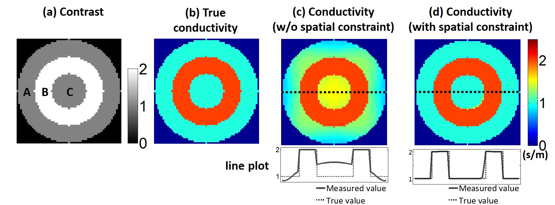
1. Simulation: For the given simulation model in Fig.2a&b, analytic solution was solved to obtain 2D-noiseless complex $$$B1^{+}map$$$. Using the phase information of $$$B1^{+}field$$$, weighted polynomial fitting (kernel size=4.3x4.3$$$cm^2$$$) was performed without and with spatial constraint.
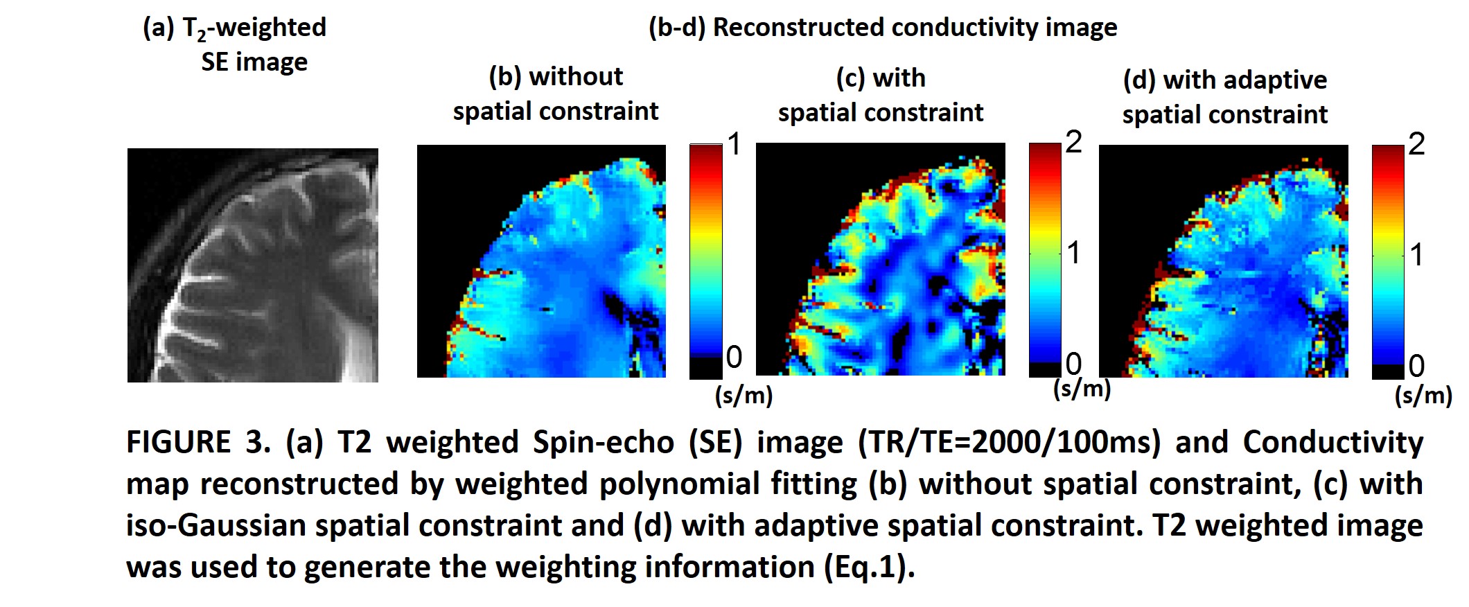
2. In-vivo experiment(Healthy volunteer): In-vivo experiments were conducted using a 3T clinical scanner (Tim Trio; Siemens Medical Solutions, Erlangen, Germany). Spin echo sequence with the following parameters was acquired : 3-mm thickness, image size = 192×192, FOV = 192×192mm,TR = 2000ms, TE=10ms, average=4 and total scan time=25.6 min. Three types of weighting scheme was evaluated. (kernel size=2.5x2.5$$$cm^2$$$)
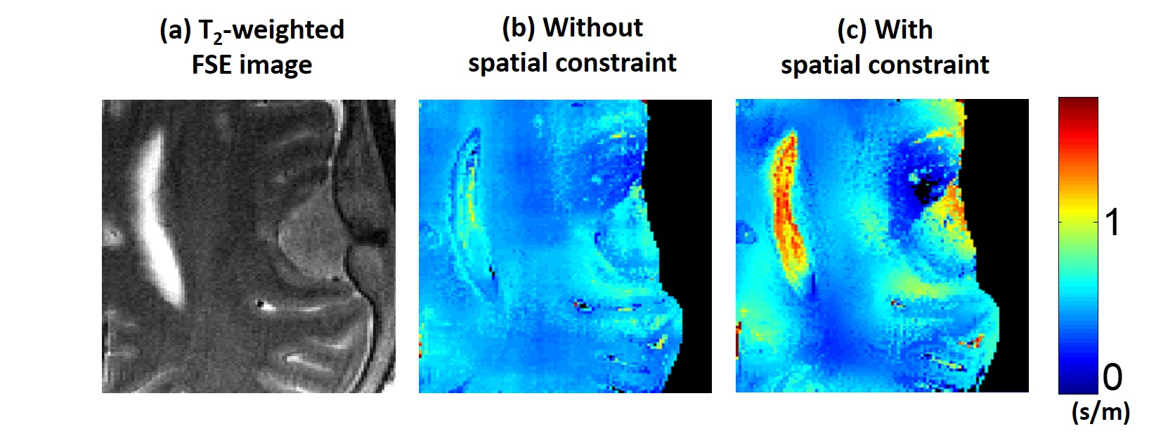
3.In-vivo experiment(meningioma): In-vivo experiments were conducted using a 3T clinical scanner (MR750, GE Healthcare, Waukesha, WI, USA). In this experiment, clinical protocol sequence that is Fast Spin-echo sequence with the following parameters was acquired : 3-mm thickness, image size=320×384, FOV=230×230mm, TR=8641ms, $$$TE_{eff} $$$=96ms, ETL=18, number of slice=50, and total scan time~20min. For patient, two types of weighting scheme was evaluated. (kernel size=4.5x4.6$$$cm^2$$$)
Result
Figure 2 presents the results of analytic simulation. Non-simply connected region was designed by inserting a material with different conductivity value (Fig.2a&b). Without spatial constraint, conductivity was under- or overestimated through the non-simply connected region (Fig.2c). In specific, over the region C, conductivity value was overestimated 48.2% (0.482S/m) in average. However, after applying spatial constraint, the error in conductivity map was reduced within 1% over whole region. Figure 3 presents the results of in-vivo experiment. The absence of spatial constraint gave underestimates (Fig.3b) comparing to the presence of spatial constraint (Fig.3c). However, due to the limited kernel size, the fixed spatial constraint shows the artificial patterns over homogeneous region (Fig.3c). Therefore, by adaptively employing spatial constraint, effective resolution of cortical region is resolved and artificial error in white matter region was reduced(Fig.3d). Conductivity map reconstructed with and without spatial constraint is shown in Fig4. Mean conductivity of meningioma is 0.5186S/m without spatial constraint and is 0.7258S/m with spatial constraint.Discussion & Conclusion
To guarantee the
accuracy of conductivity estimates, high SNR of raw data is essential. However,
in practice, it is hard to acquire high SNR data due to the time cost of data
acquisition. To resolve the limit in SNR, spatial processing is indispensable
to estimate the conductivity. In this study, spatial constraint was used to improve
the accuracy of conductivity estimates regardless of fitting kernel size. By
applying this technique to in-vivo brain, improved contrast was observed over
the cortical region, but its accuracy should be investigated in future study.
Acknowledgements
No acknowledgement found.References
1. Ulrich Katscher, Dong-Hyun Kim, and Jin Keun Seo., Recent Progress and Future Challenges in MR Electric Properties Tomography. Computational and Mathematical Methods in Medicine, vol. (2013)
2. Necip Gurler and Yusuf Ziya Ider., Gradient-based electrical conductivity imaging using MR phase. Magn Reson Med. 2016 Jan 13. doi: 10.1002/mrm.26097.
3. Kathleen M Ropella and Douglas C Noll., A Regularized Model-Based Approach to Phase-Based Conductivity Mapping. Proc. Intl. Soc. Mag. Reson. Med. 23 (2015)
4. Joonsung Lee, Jaewook Shin, and Dong-Hyun Kim., MR-based conductivity imaging using multiple receiver coils. Magn Reson Med. Volume 76, Issue 2, August 2016, Pages 530–539
Figures