Synopsis

Clarification of the contrast resolution (CR) and spatial resolution (SR) limits of phase based MREPT for conductivity imaging is essential for assessing its success success in clinical applications. Noise analysis of conventional phase based MREPT is performed to find the SNR needed for the MR sequence used for measuring B1-phase. It is found that with 1000-2000 SNR values about 0.01 S/m CR can be achieved. For SR evaluation, generalized phase based MREPT, which does not suffer from internal boundary artefacts, is considered. It is found by phantom experiments that 3.5mm spatial resolution is easily obtained with the state-of-art MR methods.

INTRODUCTION:

METHODS:

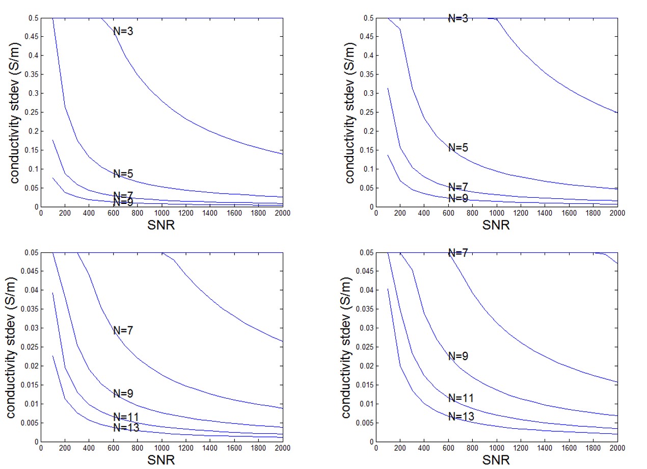
For CR evaluation we have considered conventional phase based MREPT (method1) which has the formula $$$\sigma = \frac{1}{w \mu_0}\triangledown^2 \phi$$$ where $$$\phi$$$ is the transmit B1-phase⁴. Given the approximation to the Laplacian on a Cartesian grid, $$$[\triangledown ^2(\phi)]_{i,j,k} = \frac{(\phi_{i,j,k+1} + \phi_{i,j,k-1} + \phi_{i,j+1,k} + \phi_{i,j-1,k}+ \phi_{i+1,j,k} + \phi_{i-1,j,k}) -6\phi_{i,j,k} }{(\triangle x)^2}$$$, one can find that $$$s_\sigma = \frac{1}{w \mu_0} \sqrt{\frac{6s_\phi ^2}{(\triangle x)^4} +\frac{36s_\phi ^2}{(\triangle x)^4}} = \frac{1}{w\mu_0}\frac{6.5s_\phi}{(\triangle x)^2}$$$ where $$$s_\phi$$$ is the stdev of error in the the conductivity estimate and $$$s_\sigma$$$ is the stdev of noise in the phase. It is known that $$$s_\phi=\frac{1}{SNR}$$$ where SNR is the signal-to-noise ratio of MR magnitude image³. Therefore $$$s_\sigma = \frac{1}{w\mu_0}\frac{6.5}{(\triangle x)^2} \frac{1}{SNR}$$$. Use of low pass filtering is often necessary to obtain reasonable images. If the Laplacian and the filter are cascaded then the coefficients of the overall system are to be used. In general $$$s_\sigma = \frac{1}{w\mu_0}\frac{\alpha}{(\triangle x)^2} \frac{1}{SNR}$$$ where $$$\alpha$$$ is 6.5, 0.14 or 0.21 for the cases of only Laplacian, only filter (Gaussian with N=5) or both respectively. NxNxN Gaussian filter kernels used in this study are designed to have FWHM=N/2.

For SR evaluation generalized phase based MREPT (method2) is used because it eliminates internal boundary artefacts^1,2. This method achieves conductivity reconstruction by solving the equation $$$\triangledown\phi.\triangledown\rho+ (\triangledown^2 \phi)\rho=2\omega\mu_0$$$ where $$$\rho$$$ is resistivity and $$$\phi$$$ is tranceive phase. For regularization purposes a diffusion term, $$$c\triangledown^2\rho$$$, is added to the LHS where the diffusion constant $$$c$$$ is experimentally found.

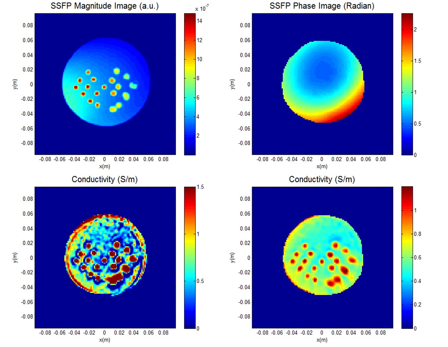
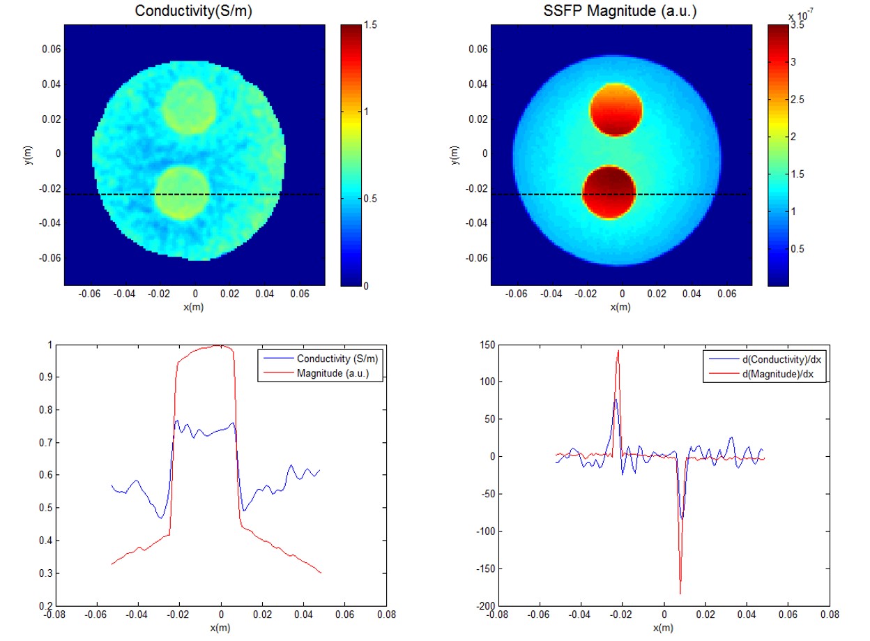
For experiments two cylindrical agar phantoms are used: SR-phantom (Figure 2) and PSF-phantom (Figure 4). SSFP sequence is used to measure B1-phase. Quadrature QBC body coil is used for transmission. For reception, QBC body coil is used for the PSF-phantom and 4-channel head coil is used for the SR-phantom.

RESULTS:

Figure 1 shows the dependence of $$$s_\sigma$$$ on N and SNR. It is observed that for voxel size of 2mmX2mmX2mm, $$$s_\sigma$$$=0.09S/m, and with N=5 we need an SNR of 600. If N=7 is used an SNR of 200 is sufficient. For N=9 and with SNR=200, $$$s_\sigma$$$=0.04S/m can be achieved. If $$$s_\sigma$$$=0.01S/m is required we need to have SNRs of 200, 300, 700, and 1700 for kernel sizes of 13, 11, 9, and 7 respectively. In 3D SSFP experiments (Figure 2) we have observed SNRs of 800 and 1600 in agar and non-agar regions where the surface coil is relatively more sensitive. In 2D SSFP experiments (Figure 4) SNRs of 200 and 400 are achieved in agar and non-agar regions uniformly across the object.

Figures 2 and 3 show the experimental results obtained with the SR-phantom. With method1 it is not possible to evaluate SR because of the internal boundary artefacts. With method2 however the 4.5mm diameter small objects are well reconstructed. The 3-3.5 mm separations between some of the objects are also identifiable. However in this case the conductivity drop in between the objects is less than 50% of the contrast of the objects themselves. With these results we can conclude that spatial resolution is about 3.5 mm.

Results with the PSF-phantom are given in Figure 4. The large homogeneous anomaly in the phantom acts as step input. The profile plot shows a sharp jump in reconstructed conductivity. When the derivative is taken the PSF is obtained. The FWHM value is about 3 pixels corresponding to 3X1.2mm=3.6mm.

DISCUSSION and CONCLUSION

We have observed that contrast resolution of 0.01S/m can be achieved with SNR such as 1700 which is experimentally possible. However if lower SNRs are obtained, then larger filter kernels must be used which means a larger homogeneous region is necessary to estimate the conductivity. For example with N=13, Gaussian filter's FWHM value is (13/2)x2mm=13mm. Regarding spatial resolution we have observed that with the experimental conditions we have in this study a spatial resolution of around 3.5 mm is indicated.

Acknowledgements

This study is supported by TUBITAK 114E522 grant. MR experiments are conducted in UMRAM, Bilkent, Ankara.

References

1. Necip Gurler and Yusuf Ziya Ider. Generalized Phase based Electrical Conductivity Imaging. Proc. Intl. Soc. Mag. Reson. Med. 24 (2016), 2991

2. Necip Gurler and Yusuf Ziya Ider. Gradient-Based Electrical Conductivity Imaging Using MR Phase. Magn. Reson. Med. Early View Version of Record online : 13 JAN 2016, DOI: 10.1002/mrm.26097

3. Scott G C, Joy M L G, Armstrong R L and Henkelman R M. Sensitivity of magnetic resonance current density imaging. J. Magn. Reson. 1992, 97 235–54

4. Ulrich Katscher, Dong-Hyun Kim, and Jin Keun Seo. Recent Progress and Future Challenges in MR Electric Properties Tomography. Computational and Mathematical Methods in Medicine,Volume 2013 (2013), Article ID 546562, 11 pages, http://dx.doi.org/10.1155/2013/546562

5. B Packham , H Koo , A Romsauerova , S Ahn , A McEwan , S C Jun and D S Holder. Comparison of frequency difference reconstruction algorithms for the detection of acute stroke using EIT in a realistic head-shaped tank. Physiol. Meas. 33 (2012) 767–786