3636
Functional connectivity mapping using 3D GRASE arterial spin labeling MRIKalen J. Petersen1, Daniel O. Claassen2, and Manus J. Donahue3
1Chemical and Physical Biology, Vanderbilt, Nashville, TN, United States, 2Neurology, Vanderbilt, 3Radiology, Vanderbilt
Synopsis
The overall goal of this work is to optimize arterial spin labeling (ASL) MRI techniques to enable the use of baseline cerebral blood flow (CBF) fluctuations to identify major intrinsically-connected resting state networks (RSNs). We provide data in support of 3D GRASE pCASL being able to provide similar functional resting state networks as BOLD. Additionally, extremely low-frequency fluctuations, less than 0.01 Hz, were present in the CBF-weighted pCASL data, suggesting that application of pCASL may provide additional functional information relative to BOLD, which generally requires low-frequency filtering.
Purpose
The goal of this work is to optimize arterial spin labeling (ASL) MRI to enable the use of baseline cerebral blood flow (CBF) fluctuations to identify major intrinsically-connected resting state networks (RSNs). While BOLD connectivity is primarily utilized for RSN analysis, BOLD suffers from major well-known limitations due to (i) susceptibility artifacts arising from the long-TE readouts, (ii) insensitivity to low-frequency (e.g., <0.01 Hz) fluctuations due to baseline drift correction procedures, and (iii) a contrast mechanism that originates from T2* changes in and around draining veins, which in many cases is not specific to regions of neuronal activity. Recently, it has been demonstrated that endogenous CBF fluctuations, measured from ASL, can also be used to identify RSNs1,2. As ASL contrast is less susceptibility-weighted, does not require baseline drift correction due to pair-wise subtraction, and originates from the capillary rather than venous vasculature, it has potential for addressing all three limitations of BOLD above. However, ASL also suffers from lower SNR and poorer temporal resolution compared to BOLD3. Here, we evaluate the ability to improve ASL RSN sensitivity by applying 3D GRASE readouts, and we contrast RSNs derived from EPI and 3D-GRASE spin labeling variants with standard BOLD approaches4.Methods
Acquisition. Healthy control (n=16; age range=24-73 years; gender=10/6 males/females) volunteers provided informed consent and were scanned at 3T (Philips Achieva). Structural T1-weighted scans (resolution=1 mm isotropic; TR/TE=8.9/4.6 ms) were acquired, along with a 10-minute baseline BOLD scan (TR/TE=2000/35 ms), and 9min 36sec 3D GRASE pCASL scan (TR=3350 ms; in-plane acceleration=3; through-plane acceleration=2; slice-oversampling=1.2; slices=20). As a reference, a pCASL 2D EPI scan (TR=4000 ms) was also acquired. Spatial resolution was matched between scans (spatial resolution=3.5 x 3.5 x 5 mm3) and pCASL scans used identical labeling duration=1550 ms and post-labeling delay=1500 ms. Analysis. BOLD scans were motion-corrected and filtered to exclude frequencies above 0.15 Hz or below 0.01 Hz (for drift correction). 4D data from the three scan types were separated into 25 spatial components by FSL MELODIC5 independent component analysis. Four candidate RSNs were then evaluated in detail: the default mode network, executive control network, visual network, and bilateral sensorimotor network, spanning a range of spatial brain regions. Curated subject-level networks were then registered to standard atlas (MNI; 2 mm) and averaged to produce group-level RSN representations for each modality. Finally, to determine if ASL yielded low-frequency information not accessible in drift-corrected BOLD data, we calculated power spectra in all scans.Results
The 3D GRASE readout improved measurement-to-measurement instability in the pCASL scans (Figure 1), with consecutive measurement instability contributing more than 20% variation for 2D EPI but less than 8% variation for 3D GRASE. Baseline BOLD and 3D GRASE ASL identified candidate networks on average (Figure 2), however, network conspicuity varied between modalities. For instance, the executive control network yielded more voxels in ASL EPI acquisitions compared to BOLD (20307 voxels vs. 8181, p<0.01). Figure 3 shows a representative DMN component for BOLD and 3D GRASE. 2D EPI pCASL was least robust for discerning independent components, and failed to identify DMN consistently. ASL and BOLD also differ in their spectral characteristics (Figure 4). The ASL data show power at low frequencies (<0.01 Hz). In contrast, the filtered BOLD data’s power goes to zero necessarily at low frequencies due to required baseline drift correction. This indicates that ASL can better extract signal from very low-frequency fluctuations than BOLD, and also that functional brain networks appear to possess non-zero low-frequency power in pCASL data.Discussion
These results suggest that BOLD and 3D GRASE pCASL MRI approaches can yield functional connectivity results broadly consistent with one another as well as with well-described networks. They also suggest that 3D readouts such as 3D GRASE are superior to traditional 2D multi-slice ASL approaches for RSN analysis, both in stability and network coherence, and capture connectivity at low frequencies better than traditional BOLD methodologies. In networks that co-localize with sensitivity to field inhomogeneity and susceptibility artifacts (e.g., executive network in frontal lobe), 3D GRASE pCASL appeared to provide more robust network detection compared to BOLD, which is likely due to differences in readout type and TE required. Other geometrical differences between networks, including the extent of involvement of outer cortical layers (e.g., Figure 2), may relate to differences in sensitivity in venous pooling between methods, and is the topic of ongoing investigation. Additionally, extremely low-frequency fluctuations, less than 0.01 Hz, were present in the CBF-weighted pCASL data, suggesting that application of pCASL may provide additional functional information relative to BOLD, which generally requires low-frequency filtering.Acknowledgements
No acknowledgement found.References
1. Dai, Weiying, et al. "Quantifying fluctuations of resting state networks using arterial spin labeling perfusion MRI." Journal of Cerebral Blood Flow & Metabolism (2015): 0271678X15615339.2. Günther, Matthias, Koichi Oshio, and David A. Feinberg. "Single-shot 3D imaging techniques improve arterial spin labeling perfusion measurements." Magnetic resonance in medicine 54.2 (2005): 491-498.
3. Xie, J., Jezzard, P., Li, L, Kong, Y., Beckman, C.F., Miller, K.L., Smith, S.M. “Identification of Resting State Networks Using Whole Brain CASL.” Abstract, ISMRM 2009.
4. Dai, Weiying, et al. "Continuous flow-driven inversion for arterial spin labeling using pulsed radio frequency and gradient fields." Magnetic Resonance in Medicine 60.6 (2008): 1488-1497.
5. Beckmann, Christian F., and Stephen M. Smith. "Probabilistic independent component analysis for functional magnetic resonance imaging." IEEE transactions on medical imaging 23.2 (2004): 137-152.
Figures
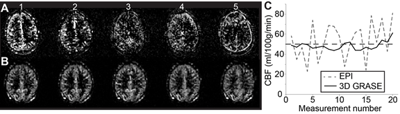
Fig. 1. Repeated measurements in the same subject using
pCASL with (A)
2D EPI readout and (B) optimized 3D GRASE readout.
Measurement-to-measurement stability with 3D GRASE is
substantially
improved, which is shown quantitatively over 20
measurements in (C). We
hypothesize that the more stable, low-frequency 3D GRASE
pCASL
fluctuations can be used for CBF-weighted functional connectivity
analysis.
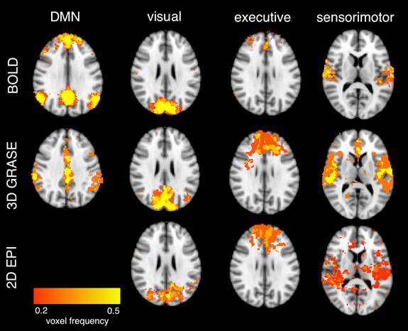
Fig 2. Averaged independent components from BOLD, 3D GRASE
pCASL, and 2D EPI pCASL reflecting the default mode network, visual network,
executive control network, and sensiorimotor regions. Color[AD1] (red to yellow) represents the fraction of individual
subject networks containing the given voxel.
[AD1]It’s
too late now, but would be better to show these from 0.2 to 1, as some of the
regions seem saturated at 0.5.
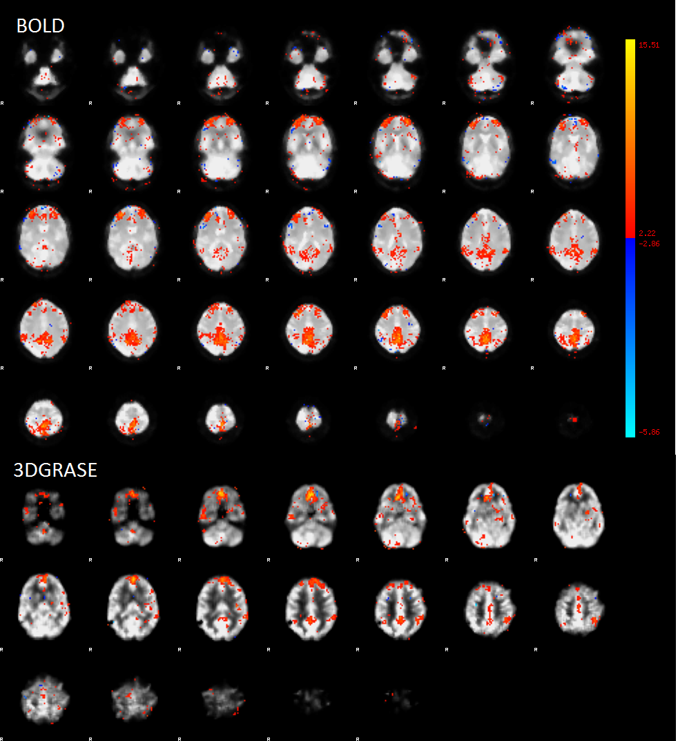
Fig 3. Single-subject images representative of default mode
network MELODIC component for BOLD and 3DGRASE ASL. Color (red to yellow)
represents z-statistic for the given voxel, thresholded at 2.22.
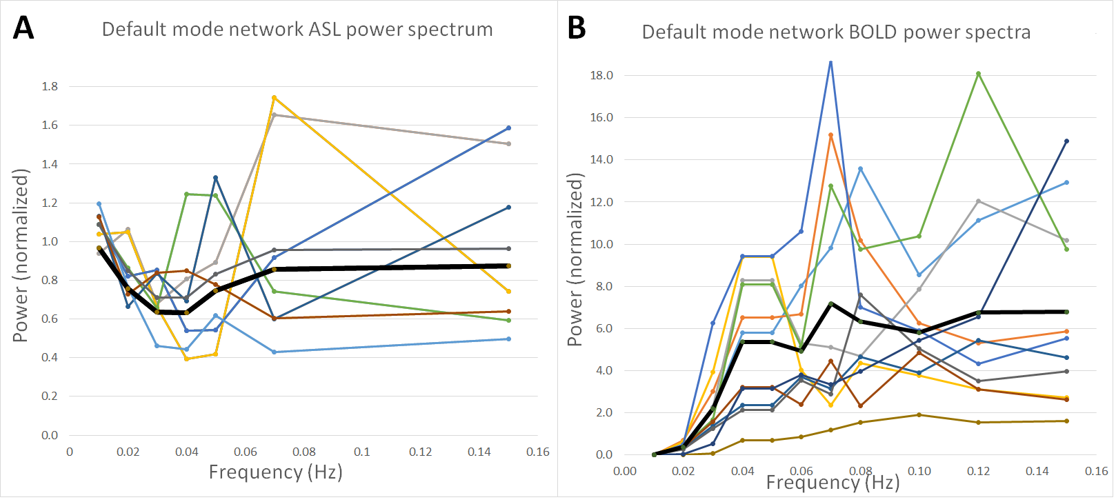
Fig 4. Power spectra at low
frequencies within the default mode network, from ASL (A) and BOLD (B) data.
Colors represent individual subjects, while black represents an average. The
power spectra were binned at 0.01 Hz intervals.