3619
Bayesian model selection of Time Encoded Arterial Spin Labelling: effect of T1 and dispersion1Department of Information Engineering, University of Padova, Padova, Italy, 2University of Verona, Verona, Italy, 3Radiology, LUMC, Gorter Center for high field MRI, Leiden, Netherlands
Synopsis
Time-Encoded Arterial Spin Labelling (TE-ASL) has been proposed as a tool to efficiently sample the kinetics of the ASL signal. We propose a model comparison based on Bayesian Model Selection (BMS), to provide insights on which is the optimal model for the quantification of TE-ASL. Our results show how important it is to consider both T1 decay and dispersion in the quantification process. When mainly interested in GM, it is advisable to incorporate the dispersion of the bolus in the model with a Gamma kernel dispersion model and to use a single T1 value of 1.3s.
Purpose
Time-Encoded Arterial Spin Labelling (TE-ASL) has been proposed as a tool to efficiently sample the kinetics of the ASL signal1. TE-ASL permits the estimation of both perfusion (CBF) and Arterial Arrival Time (AAT). We propose a model comparison based on Bayesian Model Selection (BMS), to provide insights on which is the optimal model for the quantification of TE-ASL. The model comparison will focus on the effect of T1 decay as well as dispersion of the labelled bolus on the standard Buxton model2.Methods
17 healthy controls (age 28.2±2.2) were scanned on a 3T Philips Achieva. The TE-ASL labelling scheme was optimized for T1 decay of blood1 (T1-compensated TE-ASL, 11 sub-boli, total labelling duration 3600ms, PLD 49ms, 8 averages). Readout parameters of the 2D EPI were TE/TR 22/4500ms, 17 slices, resolution of 3.75x3.75x7mm, 2 pulses of background suppression (1925 and 3120ms). Vascular crushing gradient3 with venc of 5 cm/s were used to avoid macro-vascular artefacts. A saturation recovery was acquired to quantify the T1 of tissue (T1t) and the equilibrium magnetization (M0t). T1-MPRAGE with isotropic 1mm3 resolution was acquired for co-registration. TE-ASL images were corrected for motion using a three steps linear and non-linear approach with ANTs4 and then decoded and averaged using a robust estimator to overcome the presence of outliers5. To test the influence of T1, the magnetization decay term was modified and set to either T1 of blood or T1 of Gray Matter (GM) literature values (T1b=1.65s6 and T1t=1.3s6) or to the Voxel-wise map obtained from the saturation recovery sequence (T1vw). To evaluate the effect of dispersion, each of these configurations was then combined with a no-dispersion (identity) kernel (None), or a dispersed exponential kernel7 (Exp) or a gamma kernel8 (Gamma). The resulting 9 models were tested on each subject using a Variational Bayesian (VB) estimator9. The prior information for both AAT9 and dispersion parameters were set to literature values7,8. To investigate which is the best model describing the data, we analysed the results using a Bayesian Model Selection10 (BMS) approach, approximating the model evidence with the Free Energy (FE) computed by VB. FE, CBF and AAT maps were co-registered to the T1-MPRAGE of the subject using boundary based registration method11 and normalized to an undersampled (3 mm3) version of the MNI template using ATNs4. The BMS was performed using the FE maps in the MNI space. CBF and AAT estimates of each model were compared using a within subject ANOVA (2 factors: T1 and dispersion and 3 levels respectively: T1t, T1b, T1vw and None, Exp and Gamma) using SPM12.Results
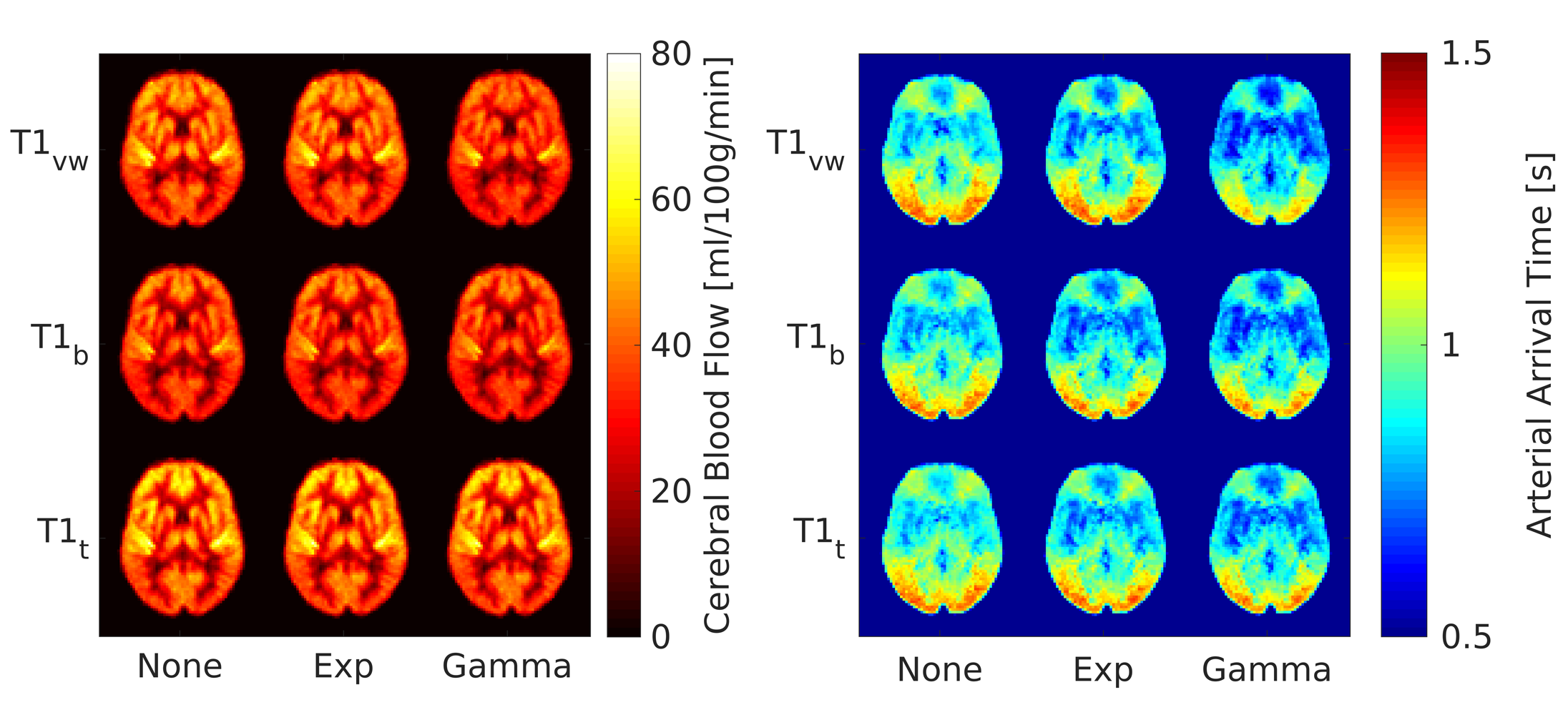
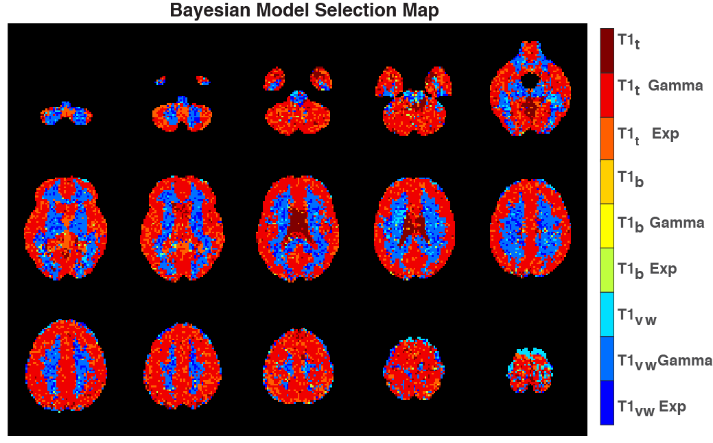
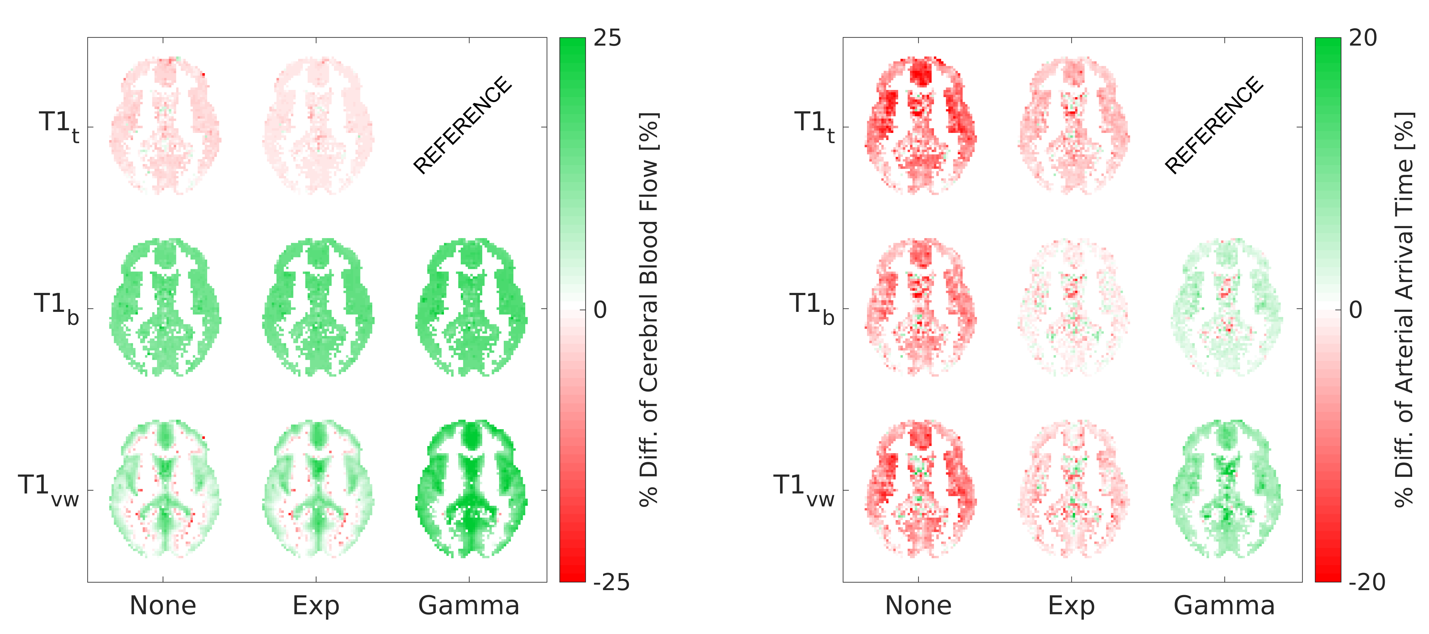
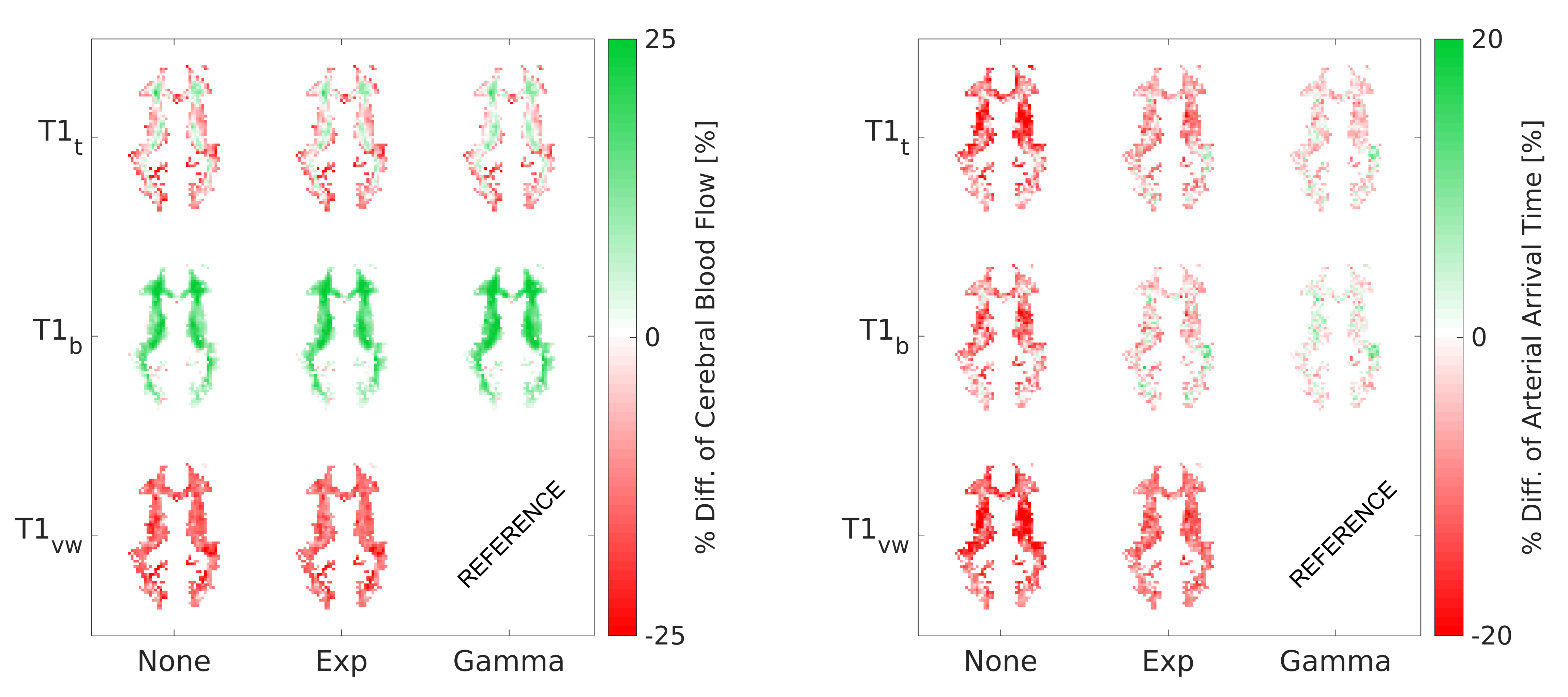
Fig.1 shows a representative slice of the group mean CBF and AAT for each model. The BMS analysis (Fig. 2) highlighted that the combination of T1t-Gamma is the more probable model in 80.1% of the GM voxels. When extending the analysis to the whole brain, BMS pointed out that in non GM regions the more probable model was the T1vw-Gamma (77.3%). The mean percentage differences in CBF and AAT between the selected model for the GM (T1t-Gamma) or other tissues (T1vw-Gamma) and the other tested models are showed in Fig.3 and Fig.4 respectively. The statistical analysis showed for both CBF and AAT a statistically significant main effect of both T1 and dispersion (FWE corrected with α=0.05). Moreover, the ANOVA showed no significant interaction between T1 and dispersion.Discussion
BMS analysis suggested different optimal models for CBF-quantification in a large portion of GM and WM voxels. Moreover, a subsequent statistical analysis showed that the effect of the choice of the optimal T1 seems to play a major role in CBF quantification. More subtle, but not negligible, is the effect of dispersion on CBF. On the contrary, AAT is more effected by dispersion than T1. When mainly interested in GM, it seems best to use a fixed value for T1. Moreover, the effect of this choice on CBF and AAT in WM is only moderate. The sub-optimal performance in GM when using T1vw might be due to partial volume effects of the low-resolution saturation recovery acquisition employed.Conclusion
Our results show how important it is to consider both T1 decay and dispersion in the quantification process. When mainly interested in GM of healthy controls, the suggested model is T1t-Gamma. Therefore, it is advisable to incorporate the dispersion of the bolus in the model with a Gamma kernel dispersion model and to use a single T1 value of 1.3s.Acknowledgements
No acknowledgement found.References
1. Teeuwisse WM, Schmid S, Ghariq E, Veer IM, van Osch MJP. Time-encoded pseudocontinuous arterial spin labeling: Basic properties and timing strategies for human applications. Magn Reson Med. 2014;1722:1712-1722.
2. Buxton RB, Frank LR, Wong EC, Siewert B, Warach S, Edelman RR. A general kinetic model for quantitative perfusion imaging with arterial spin labeling. Magn Reson Med. 1998;40(3):383-396.
3. Ye FQ, Mattay VS, Jezzard P, Frank JA, Weinberger DR, McLaughlin AC. Correction for vascular artifacts in cerebral blood flow values measured by using arterial spin tagging techniques. Magn Reson Med. 1997;37(2):226-235.
4. Avants BB, Epstein CL, Grossman M, Gee JC. Symmetric diffeomorphic image registration with cross-correlation: Evaluating automated labeling of elderly and neurodegenerative brain. Med Image Anal. 2008;12(1):26-41.
5. Maumet C, Maurel P, Ferré J-C, Barillot C. Robust estimation of the cerebral blood flow in arterial spin labelling. Magn Reson Imaging. 2014;32(5):497-504.
6. Alsop DC, Detre JA, Golay X, et al. Recommended implementation of arterial spin-labeled perfusion MRI for clinical applications: A consensus of the ISMRM perfusion study group and the European consortium for ASL in dementia. Magn Reson Med. April 2014.
7. Meyer E. Simultaneous correction for tracer arrival delay and dispersion in CBF measurements by the H215O autoradiographic method and dynamic PET. J Nucl Med. 1989;30(6):1069-1078.
8. Chappell MA, Woolrich MW, Kazan S, Jezzard P, Payne SJ, MacIntosh BJ. Modeling dispersion in arterial spin labeling: validation using dynamic angiographic measurements. Magn Reson Med. 2013;69(2):563-570.
9. Chappell M a, Groves a R, Whitcher B, Woolrich MW. Variational Bayesian Inference for a Nonlinear Forward Model. IEEE Trans Signal Process. 2009;57(1):223-236.
10. Rigoux L, Stephan KE, Friston KJ, Daunizeau J. Bayesian model selection for group studies - Revisited. Neuroimage. 2014;84:971-985.
11. Greve DN, Fischl B. Accurate and robust brain image alignment using boundary-based registration. Neuroimage. 2009;48(1):63-72.
Figures