3542
Multi compartment deconvolution with L2 regularization and priors improves repeatability of MD estimation through free water and IVIM elimination.1Department of Information Engineering, University of Padova, Padova, Italy, 2Neuroimaging Lab, Scientific Institute IRCCS Eugenio Medea, Bosisio Parini (LC), Italy, 3Radiology Department, University Medical Center Utrecht, Utrecht, Netherlands
Synopsis
Pseudo continuous description of the diffusion MRI (dMRI) signal through multi-compartment deconvolution is a promising technique to disentangle different water pools in the brain. In this work we verified whether a deconvolution based approach with L2 regularized priors could improve the repeatability of DTI metrics computed on the brain data of 3 volunteers acquired twice. Signal fractions of free water and perfusion could reliably be quantified and removed from the diffusion signal, improving the repeatability of MD estimation both in gray and white matter.
Purpose
Pseudo continuous description of the diffusion MRI (dMRI) signal through multi-compartment deconvolution[1] is a promising technique to disentangle different water pools in the brain. In this work we aim to verify whether such approach could improve the repeatability of DTI metrics, while simultaneously providing a number of additional parameters.Methods
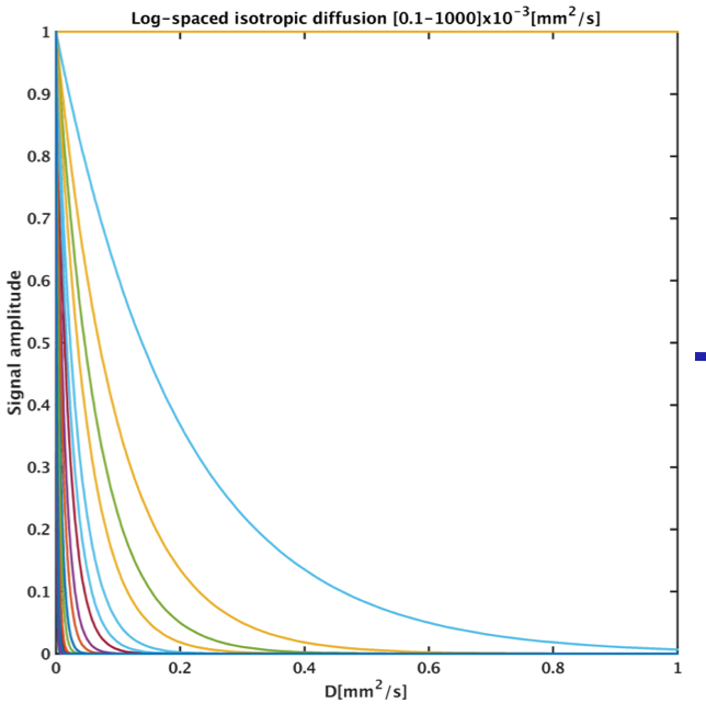
A dictionary of 300 mono-exponential Gaussian decaying signals with diffusion coefficients log-spaced in the range [0,1000]µm2/ms was defined. Membrane restrictions essentially cause the dMRI signal not to decay at strong diffusion weightings, therefore their effect can be modeled with the addition of a constant column to the dictionary, as shown in Figure 1. Deconvolution is inherently noisy, thus we developed a three stage solution. Firstly, L2 regularized Non-Negative Least Squares (NNLS) were applied to obtain the voxel-wise deconvolution spectra of each subject. These were averaged and used to define a deconvolution prior(χ0). The second deconvolution step was performed minimizing voxel-wise the following terms:
$$min||Uχ-S||_2^2+||γχ-χ_0||_2^2$$
$$Uχ≥0$$
where χ is the diffusion spectra, U the deconvolution dictionary, S the dMRI signal and γ a regularization term. L2 regularization may bias the estimation of the signal amplitudes, thus as last step the diffusion dictionary was voxel-wise reduced to its minimal components (non-zero diffusion coefficients in the previous step), then the final NNLS deconvolution was performed. The voxel-wise diffusion spectra were integrated in specific diffusion ranges to obtain fractional maps: IVIM for diffusion values in the range [6,500]µm2/ms, Free Water (FW) in the range [2.5,6]µm2/ms and non-Gaussian (NG) in the range [0,0.4] µm2/ms. 3 healthy controls (HC, 1 male, 27±1 years) were acquired twice at 3T with 7 days inter-scan. The acquisition protocol included a T1W scan (1mm3 resolution, TE/TR=3.7/8.1ms), a T2W scan (1.5x1.5x1.5mm3 resolution, TE/TR=0.1/4.2s) and a dMRI sequence (2.5x2.5x2.5mm3 resolution, TE/TR=80ms/6.9s). dMRI data was pre-processed with Tortoise[2] using the T2W as reference. Mean diffusivity was derived from the linear DTI fit of the data at b=5,1000s/mm2 before(MD) and after(MDC) subtraction of the FW and IVIM components (referred as corrected DTI). T1W data was segmented[3], [4], then boxplots of MD/MDC, NG, FW and IVIM were computed individually within the GM and WM of each time-point. Repeatability of MD/ MDC was assessed with Intra-Class Correlation(ICC).
Results
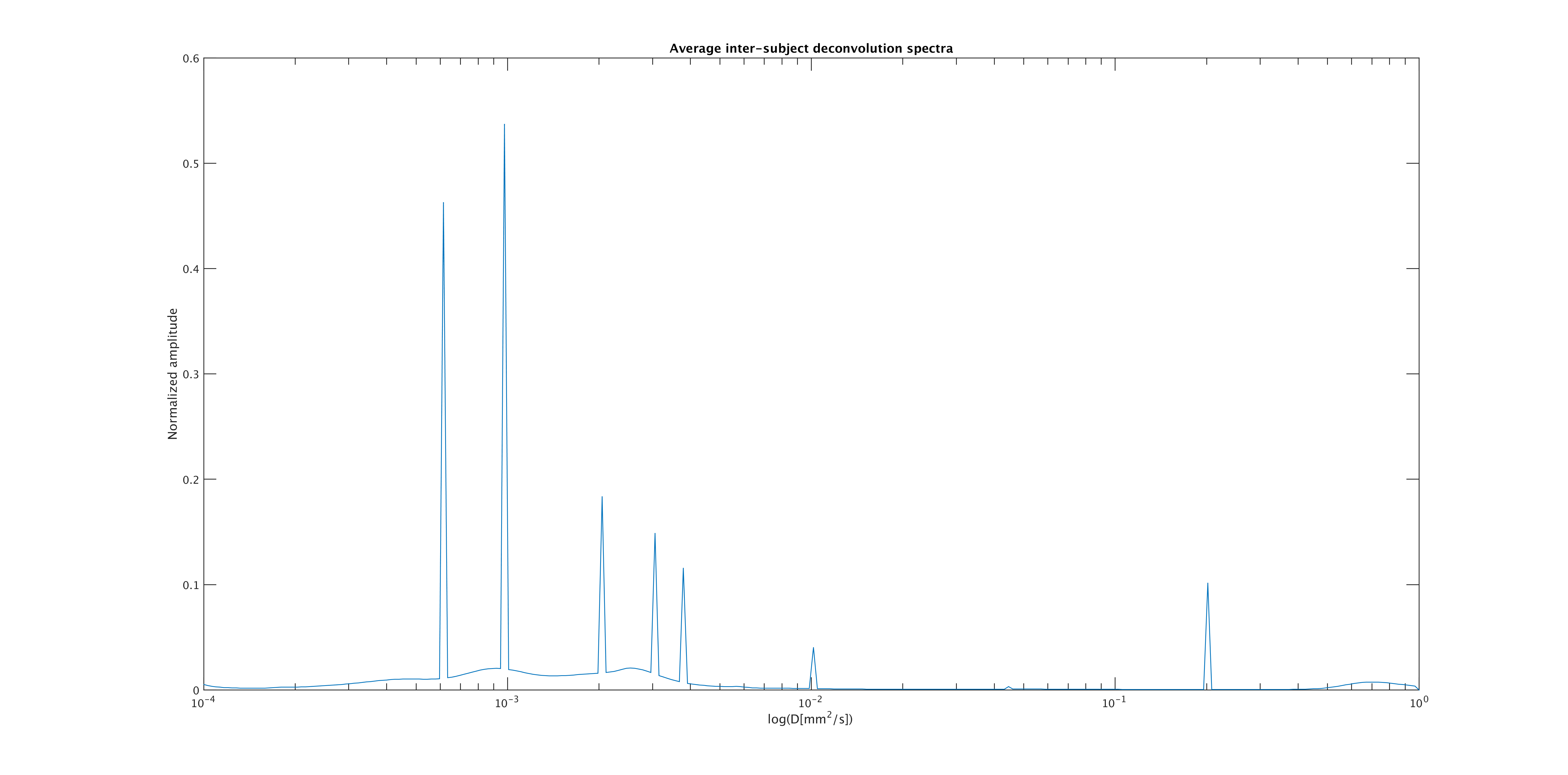
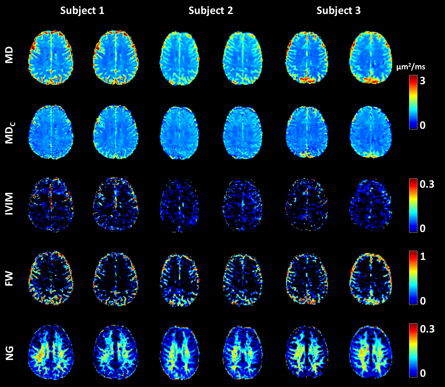
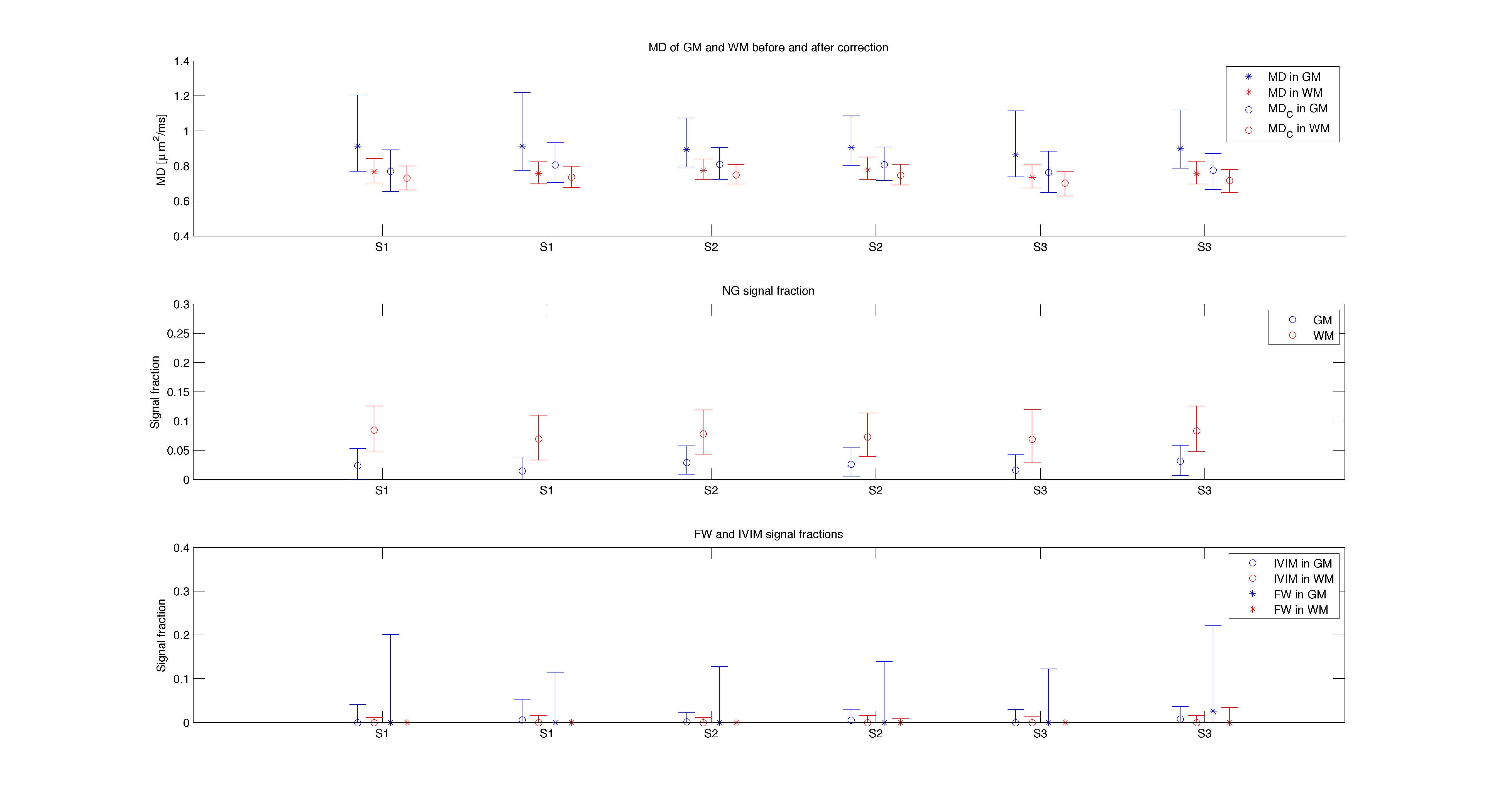
Figure 2 shows the deconvolution spectra obtained averaging the results of the voxel-wise L2 regularized NNLS of each subject. Seven diffusion peaks were revealed at [0.6,1.0,2.0,3.0,3.8,10.1,200.5]µm2/ms. An additional peak at zero-diffusion (NG) was also observed. The deconvolution prior was defined accordingly but discarding the peaks at 1.0 and 3.8 µm2/ms. Figure 3 shows an axial slice of the fractional IVIM, FW and NG maps obtained by integration of the voxel-wise deconvolution spectra, as well as maps of MD from the corrected and uncorrected DTI fits. IVIM and FW had higher values in GM compared to WM. IVIM, FW and NG maps were similar across time-points, with NG assuming higher values in WM, as expectable. MDC maps were more flat and lowered values than MD. 25, 50 and 75 percentile of MD/MDC, NG, FW and IVIM are reported in Figure 4. MD assumed values between 0.73 and 1.22µm2/ms in GM, between 0.67 and 0.85µm2/ms in WM. MDC values ranged between 0.65 and 0.94µm2/ms in GM, between 0.63 and 0.81µm2/ms in WM. ICC of MD were 0.69 and 0.84 for GM and WM respectively, values that increased to 0.75 and 0.95 for MDC. Both estimated FW and IVIM contributions were higher in GM than WM, although IVIM fractions were below 5%. The average NG fractions were 7.6% and 2.3% for WM and GM respectively.Discussion
The values of MD/MDC,FW and IVIM were different for GM and WM. L2 regularized NNLS with priors improved the repeatability of MD estimates, with ICC values of MDC up to 0.95 in WM. IVIM fractions were in line with generally accepted values and below 10%. FW values were higher and up to 20%, eventually due to partial volume effects at the CSF interface. Despite the consistent results, further investigation of the stability of the algorithm is required given the limited analyzed sample.Conclusions
We propose an approach to perform multi-compartment deconvolution of the dMRI data, estimating signal contributions from multiple diffusion regimes. Our three stage pipeline limited the inherent variability of the deconvolution operation and improved the repeatability of MD estimates in the brain.Acknowledgements
No acknowledgement found.References
[1] B. Madler, D. R. Hadizadeh, and J. Gieseke, “Assessment of a Continuous Multi-Compartmental Intra-Voxel Incoherent Motion ( IVIM ) Model for the Human Brain,” in International Society for Magnetic Resonance in Medicine, 2013.
[2] C. Pierpaoli, L. Walker, M. O. Irfanoglu, A. S. Barnett, P. J. Basser, L.-C. Chang, C. G. Koay, S. Pajevic, G. K. Rohde, J. Sarlls, and M. T. Wu, “TORTOISE: an integrated software package for processing of diffusion MRI data,” ISMRM 18th Annu. Meet., p. 1597, 2010.
[3] S. M. Smith, “Fast robust automated brain extraction.,” Hum. Brain Mapp., vol. 17, no. 3, pp. 143–55, Nov. 2002.
[4] Y. Zhang, M. Brady, and S. Smith, “Segmentation of brain MR images through a hidden Markov random field model and the expectation-maximization algorithm.,” IEEE Trans. Med. Imaging, vol. 20, no. 1, pp. 45–57, Jan. 2001.
Figures