3541
Bias Field Correction and Intensity Normalisation for Quantitative Analysis of Apparent Fibre Density1Florey Institute of Neuroscience, Melbourne, Australia, 2Centre for the Developing Brain, Division of Imaging Sciences and Biomedical Engineering, Kings College London, London, United Kingdom
Synopsis
Apparent Fibre Density (AFD) is a measure derived from un-normalised fibre orientation distributions. To make AFD quantitative across subjects, images need to be intensity normalised and bias field corrected. Here we present a fast and robust approach to simultaneous bias field correction and intensity normalisation by exploiting tissue compartment maps derived from multi-tissue constrained spherical deconvolution. We performed simulations to show that the method can accurately recover a ground truth bias field, while also demonstrating qualitative results on in vivo data.
Purpose
A new method for bias field correction and intensity normalisation to enable quantitative comparison of apparent fibre density.Introduction
Apparent Fibre Density (AFD) is a Fibre Orientation Distribution-derived measure developed to enable fibre-specific quantitative analysis using HARDI data1. While most DWI models derive quantitative measures by normalising the DW signal to the b=0 signal within each voxel, issues arise when all compartments within the voxel (and their T2s) are not modelled appropriately (i.e. CSF, GM, extra-axonal space, myelin)2,3. In contrast, previous AFD studies4 have relied on global intensity normalisation (based on the median CSF or WM b=0s/mm2 value), following bias field correction (with the field estimated from the b=0s/mm2 image). This approach is not ideal since: 1) intensity normalisation using the median CSF or WM b=0s/mm2 value may be biased when pathology is extensive or influences the selection of exemplar voxels for intensity normalisation; 2) the similar T2w values for GM and WM make histogram-based bias field estimation difficult.
Here we propose a fast and robust method for simultaneous intensity normalisation and bias field correction of DWI data by exploiting information derived from multi-tissue constrained spherical deconvolution (mtCSD)5,6.
Methods
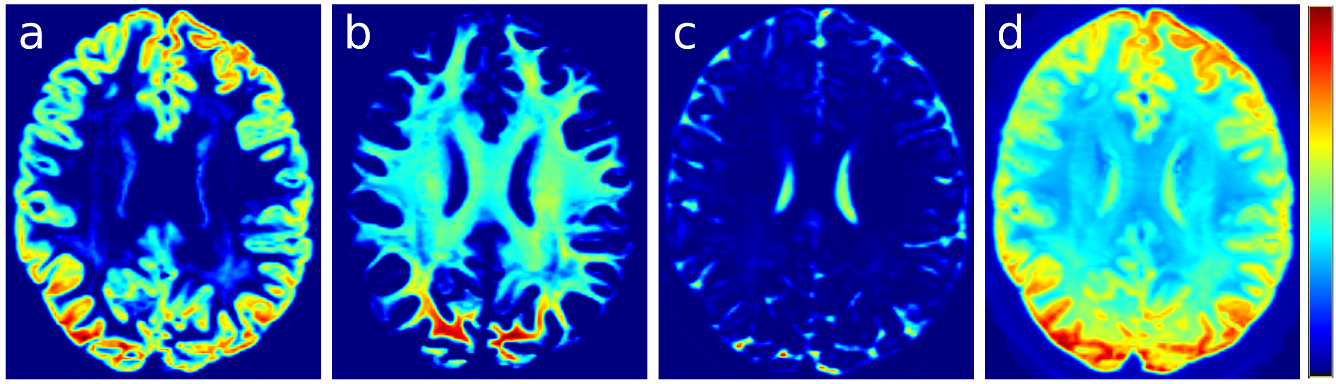
All brain voxels contain either GM, WM or CSF (or some mixture thereof); ideally, therefore, the tissue compartment maps from mtCSD should sum to 1. In practice, variations in T2 will mean that the compartment weights do not generally sum to 1. While a unit sum constraint could be imposed on the output of mtCSD, in practice the method operates without any form of voxel-wise normalisation to ensure linearity of the estimated volume fractions with respect to the measured DW signal. Consequently, the output tissue compartment maps are also affected by intensity variations due to the bias field (Fig. 1a-c). Furthermore, because the response functions used in the mtCSD are estimated from a subset of voxels in each tissue class7, the magnitude of the response functions may not be appropriate for the whole brain, leading to tissue-specific hyper- or hypo-intensities in the summed image (GM+GM+CSF) (Fig. 1d).
We estimate a bias field and a global scale factor per tissue type $$$s_{t}$$$ by minimising the cost function, $$$F$$$:
$$F(\mathbf{w},\mathbf{s})=\int_{\Omega}|1−\frac{\sum_{t=1}^{m}s_{t}C_{t}(x)}{\mathbf{w}^{T}B(x)}|^{2}dx$$
where the bias field is modelled by polynomial basis functions $$$B(x)$$$ at voxel $$$x$$$ with weights $$$\mathbf{w}$$$. $$$C_{t}(x)$$$ is the value of the compartment density map for tissue $$$t$$$ , $$$m$$$ is the number of tissue compartments, and $$$s_{t}$$$ is used to account for global differences in magnitude between tissue types due to miscalibrated response function magnitudes.
To minimise $$$F$$$, we iterate between performing a least squares solve for a vector containing the global scale factors $$$\mathbf{s}$$$ (given the current estimate of $$$\mathbf{w}$$$), and a least squares solve for $$$\mathbf{w}$$$ (given the current estimate of $$$\mathbf{s}$$$), normalising the bias field to average 1 in all brain mask voxels. Optimisation is stopped at convergence (~5 iterations).
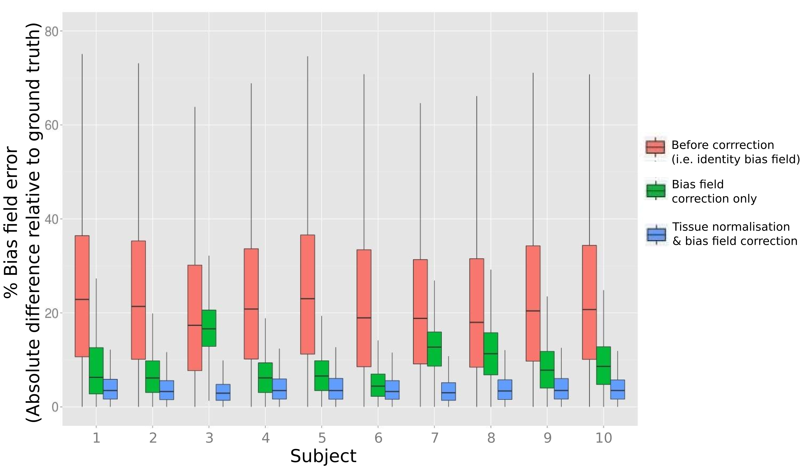
To evaluate the proposed method, we applied 10 different “ground truth” bias fields to a bias-field-free diffusion MRI phantom8. The ground truth fields were obtained from 10 different subjects from the human connectome project (HCP)9. We then performed mtCSD using GM, WM and CSF response functions that were randomly scaled by a factor (range 0.8-1.2) to simulate miscalibration of the response functions. We performed two experiments: 1) estimation of the bias field (i.e. no intensity normalisation by $$$\mathbf{s}$$$) 2) Estimating the bias field and intensity normalisation. Results were evaluated by computing the error at each voxel as the absolute difference between the estimated field and the ground truth, expressed as percentage of the ground truth.
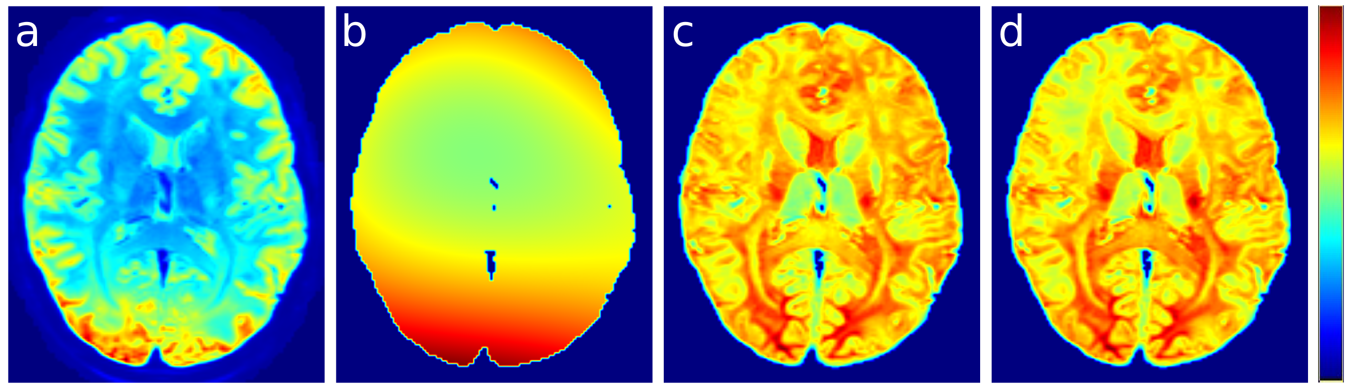
We also demonstrate the proposed method on an in vivo dataset, using tissue maps obtained from mtCSD of a single HCP subject, and visually compare the result to a commonly used approach10.
Results
As shown by Fig 2, for all 10 simulations the median error for all voxels in the brain mask was substantially reduced when modelling the bias field from the summed tissue compartment image. When also estimating tissue normalisation scale factors to account for the effect of miscalibration in response function magnitudes, the error in the estimated field was further reduced. Fig. 3 demonstrates that in real in vivo data, the proposed method produces a map of summed tissue densities that is more homogeneous (and hence more biologically realistic) than the N4-based approach10.Discussion and Conclusion
We have demonstrated a fast a robust method for simultaneously correcting the bias field and performing global intensity normalisation of mtCSD compartment maps. The corrected tissue maps may be subsequently used for direct quantitative analysis (e.g. fixel-based analysis4) or connectivity studies11.Acknowledgements
No acknowledgement found.References
1. Raffelt D, Tournier J-D, Rose S, Ridgway GR, Henderson R, Crozier S, et al. Apparent Fibre Density: a novel measure for the analysis of diffusion-weighted magnetic resonance images. Neuroimage 2012;59:3976–3994.
2. Berlot R, Metzler-Baddeley C, Jones DK, O’Sullivan MJ. CSF contamination contributes to apparent microstructural alterations in mild cognitive impairment. Neuroimage 2014;92:27–35.
3. Bouyagoub S, Dowell N, Hurley S, Wood T, Cercignani mara. Overestimation of CSF Fraction in NODDI: Possible Correction Techniques and the Effect on Neurite Density and Orientation Dispersion Measures. In: Proc. Int. Soc. Magn. Reson. Med. Singapore: 2016.
4. Raffelt DA, Tournier J-D, Smith RE, Vaughan DN, Jackson G, Ridgway GR, et al. Investigating white matter fibre density and morphology using fixel-based analysis. Neuroimage 2016;
5. Jeurissen B, Tournier J-D, Dhollander T, Connelly A, Sijbers J. Multi-tissue constrained spherical deconvolution for improved analysis of multi-shell diffusion MRI data. Neuroimage 2014;103:411–426.
6. Dhollander T, Connelly A. A novel iterative approach to reap the benefits of multi-tissue CSD from just single-shell (+b=0) diffusion MRI data. Proc ISMRM 2016;24:3010.
7. Dhollander T, Raffelt D, Connelly A. Unsupervised 3-tissue response function estimation from single-shell or multi-shell diffusion MR data without a co-registered T1 image. Proc ISMRM Workshop on Breaking the Barriers of Diffusion MRI 2016:5.
8. Esteban O, Caruyer E, Daducci A, Bach-Cuadra M, Ledesma-Carbayo MJ, Santos A. Diffantom: Whole-Brain Diffusion MRI Phantoms Derived from Real Datasets of the Human Connectome Project. Front. Neuroinform 2016;4.
9. Van Essen DC, Ugurbil K, Auerbach E, Barch D, Behrens TEJ, Bucholz R, et al. The Human Connectome Project: a data acquisition perspective. Neuroimage 2012;62:2222–2231.
10. Tustison NJ, Avants BB, Cook PA, Zheng Y, Egan A, Yushkevich PA, et al. N4ITK: improved N3 bias correction. IEEE Trans Med Imaging 2010;29:1310–1320.
11. Smith RE, Tournier J-D, Calamante F, Connelly A. SIFT: Spherical-deconvolution informed filtering of tractograms. Neuroimage 2013;67:298–312.
Figures