3533

A unified framework for upsampling and denoising of diffusion MRI data

Samuel St-Jean¹, Max Viergever¹, and Alexander Leemans¹

¹Image Sciences Institute, University Medical Center Utrecht, Utrecht, Netherlands

Synopsis

Diffusion MRI suffers from relatively long scan times and low signal to noise ratio (SNR), which limits the acquired spatial resolution. In this work, we propose a unified framework for denoising and upsampling diffusion datasets based on a sparse representation of the diffusion signal. Our proposed method shows less blurring and increased anatomical details in the pons region when compared to denoising and subsequent spline interpolation. At the junction of the corpus callosum, the corticospinal tract and the cingulum, finer structures are also preserved as evidenced by a high resolution invivo acquisition.

Introduction

Diffusion MRI (dMRI) suffers from relatively long scan times and low signal to noise ratio (SNR), which limits the acquired spatial resolution. Many techniques have emerged to increase image quality and achieve higher spatial resolutions such as specialized acquisition schemes^{1, 2, 3}, image processing techniques to increase spatial resolution^4,5,6 and denoising techniques to increase the SNR^7,8,9. While these methods typically aim to either increase the spatial resolution or improve the SNR, it would be beneficial to combine both, enhancing their effectiveness. In this work, we propose such a unified framework for denoising and upsampling dMRI data based on a sparse representation of the diffusion signal.

Theory

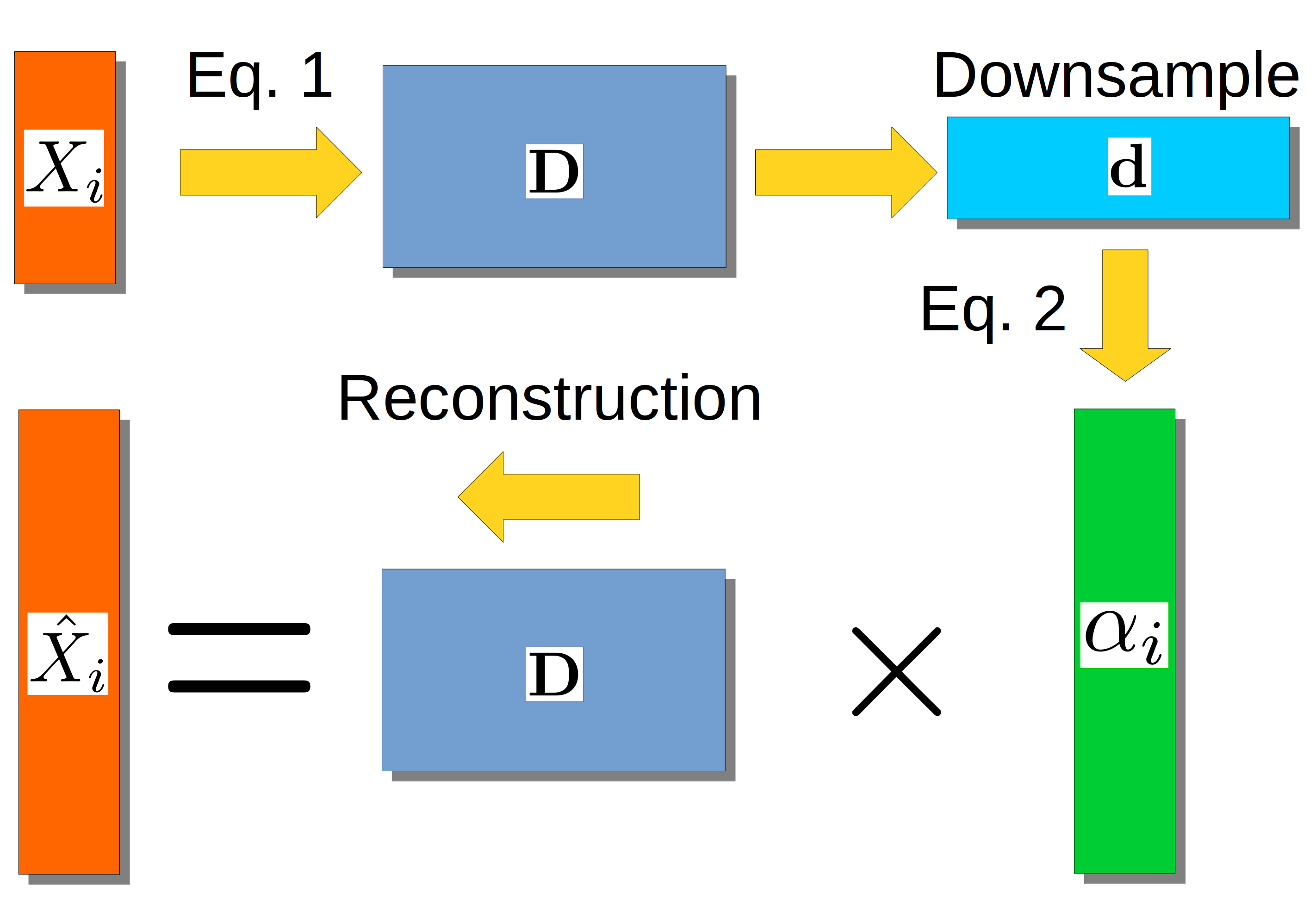
Sparse linear models have been used as a powerful method to represent the MRI signal by only using a few elements. Such a representation has been used for structural MRI upsampling¹⁰ or dMRI denoising⁸. The key idea is to decompose locally $$$n$$$ dMRI signals $$$X_i$$$ as a linear combination of a few basis elements¹¹ through equation 1. By exploiting the redundancy of the signal, a sparse representation $$$\hat{X}_i=\textbf{D}\alpha_i$$$ can be found, with $$$X_i$$$ the MRI signal in a neighborhood $$$i$$$, $$$\textbf{D}$$$ the dictionary, $$$\alpha_i$$$ the sparse coefficients, $$$\lambda$$$ a tradeoff parameter between data fitting and sparsity and $$$\hat{X}_i$$$ the reconstructed signal.

$$\text{Equation 1}\enspace\min_{\mathbf{D},\alpha}\frac{1}{n}\sum_{i=1}^n\left(\frac{1}{2}\|X_i-\mathbf{D}\alpha_i\|_2^2+\lambda\|\alpha_i\|_1\right)\enspace\text{s.t.}\enspace\|\mathbf{D}\|_2^2=1$$

In our unified framework, we propose to extract a lower resolution representation $$$\textbf{d}$$$ by averaging the columns of $$$\textbf{D}$$$ to form smaller patches, thus giving a one-to-one mapping between low and high resolutions patches within a multiscale approach¹². We then solve equation 2 using $$$\textbf{d}$$$ with $$$\lambda_i=\sigma^2_i(m+3\sqrt{2})$$$ and $$$m$$$ the number of elements in a patch. This would give a denoised representation⁸ for $$$\hat{X}_i=\textbf{d}\alpha_i$$$, but by instead using the direct relationship between $$$\textbf{d}$$$ and $$$\textbf{D}$$$, we reconstruct a high resolution, denoised representation $$$\hat{X}_i=\textbf{D}\alpha_i$$$ as shown schematically in figure 1.

$$\text{Equation 2}\enspace\min_{\alpha_i}\|\alpha_i\|_1\enspace\text{s.t.}\enspace\frac{1}{2}\|X_i-\mathbf{d}\alpha_i\|_2^2\le\lambda_i$$

Methods

Two datasets of the same subject were obtained on the same 3T Philips scanner; a 1.8 mm dataset with $$$64\thinspace\text{b}=1000\thinspace\text{s/mm}^2$$$ volumes, $$$\text{TR/TE}=18.9\thinspace\text{s}\thinspace/\thinspace104\thinspace\text{ms}$$$ and a 1.2 mm dataset with $$$40\thinspace\text{b}=1000\thinspace\text{s/mm}^2$$$ volumes, $$$\text{TR/TE}=11.1\thinspace\text{s}\thinspace/\thinspace63\thinspace\text{ms}$$$, both with one $$$\text{b}=0\thinspace\text{s/mm}^2$$$ volume. The 1.2 mm dataset serves as a gold standard for spatial resolution attainable with enough signal within a reasonable timeframe on a standard scanner.

Using the 1.8 mm dataset, we first estimated the variance of the Rician noise with PIESNO¹³ and corrected for Rician noise bias¹⁴. We extracted spatial patches of size (6,6,6) with 5 angular q-space neighbors to construct $$$\textbf{D}$$$ using equation 1 and then downsampled $$$\textbf{D}$$$ by a factor of 2 in each dimension, thus creating $$$\textbf{d}$$$ of size (3,3,3). The coefficients $$$\alpha_i$$$ were computed with equation 2 and $$$\textbf{d}$$$, thus obtaining an upsampled $$$\hat{X}_i=\textbf{D}\alpha_i$$$ at 0.9 mm. To show the improvements of the proposed method, we denoised separately the 1.8 mm and 1.2 mm datasets. The original 1.8 mm and denoised datasets were then upsampled by a factor 2 using both linear spline and cubic spline interpolation as described previously⁵. We also computed colored fractional anisotropy (FA) maps with a robust tensor estimation¹⁵ as implemented in ExploreDTI¹⁶.

Results

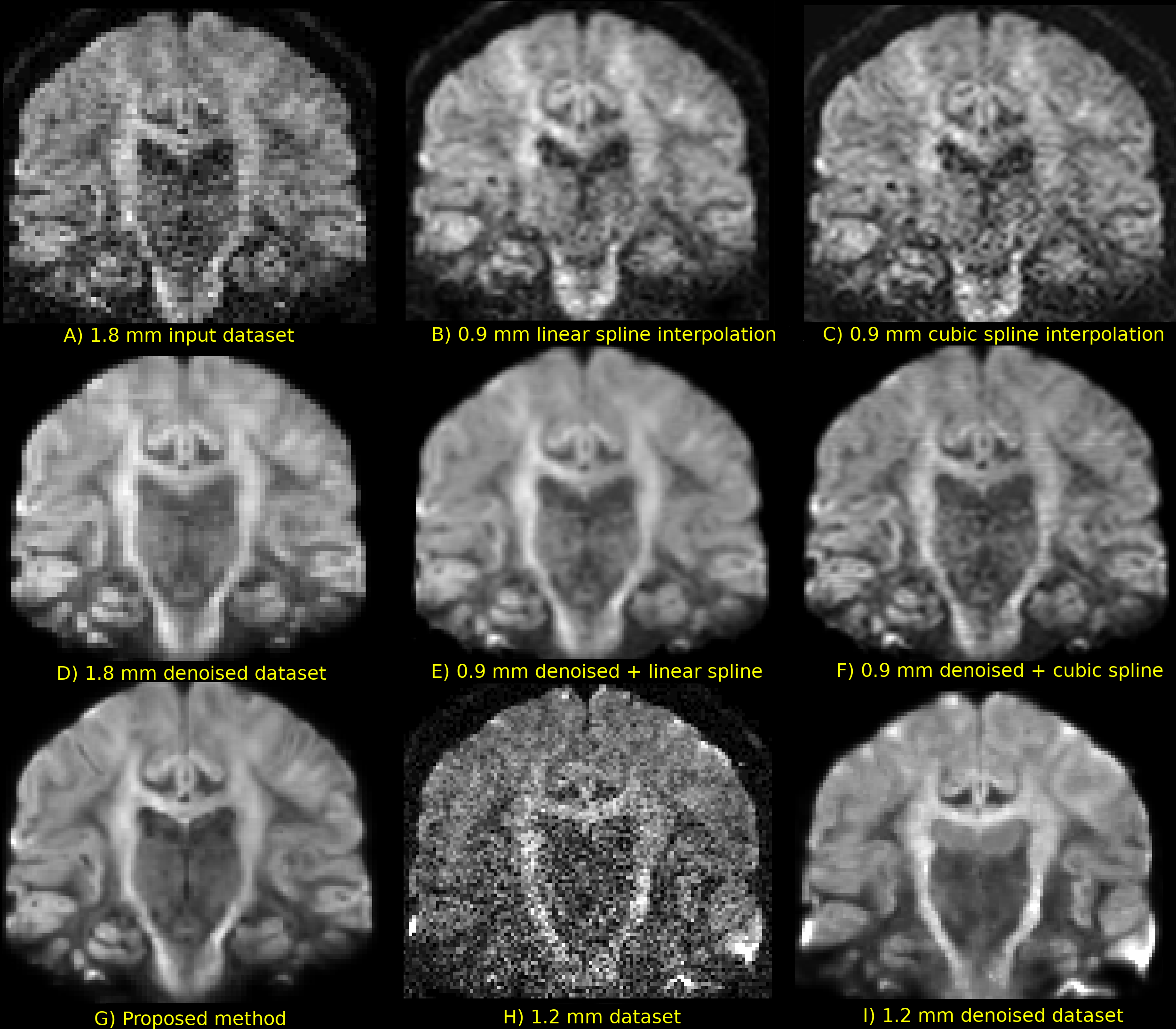
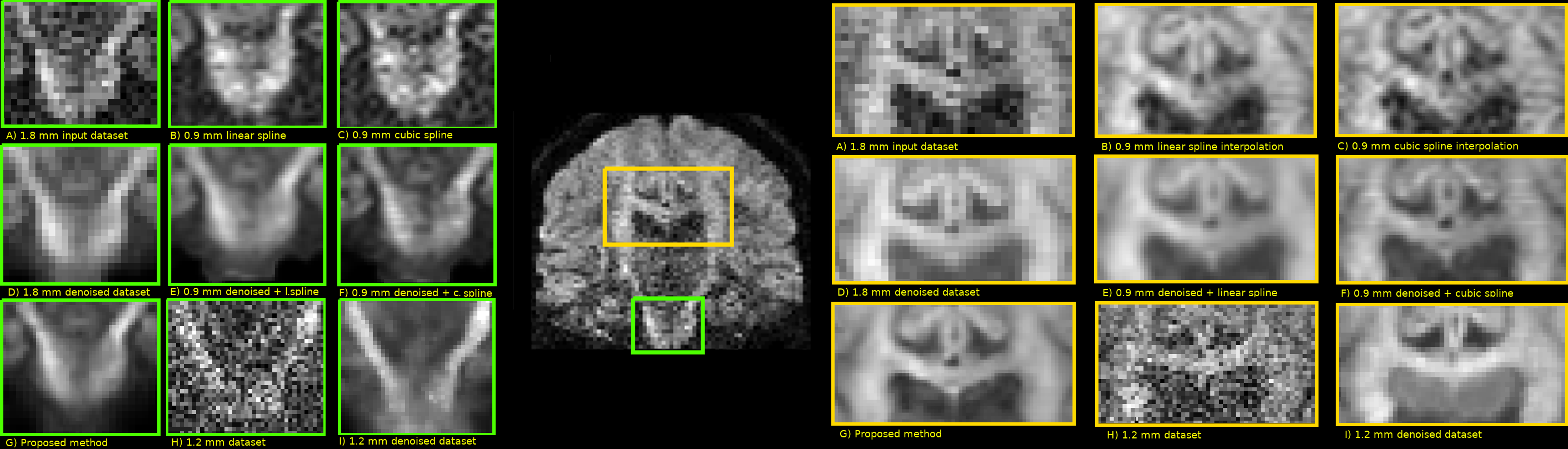
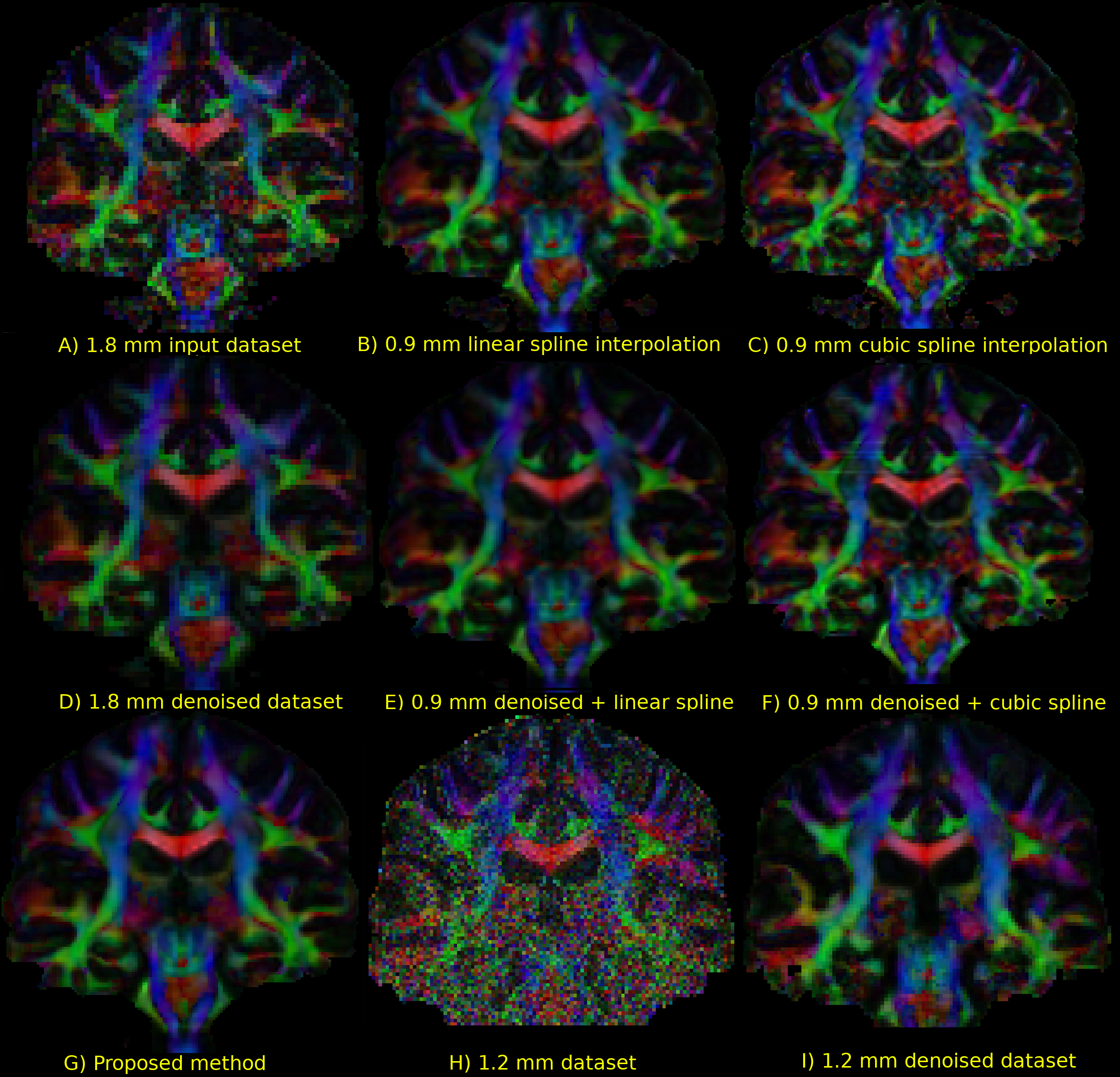
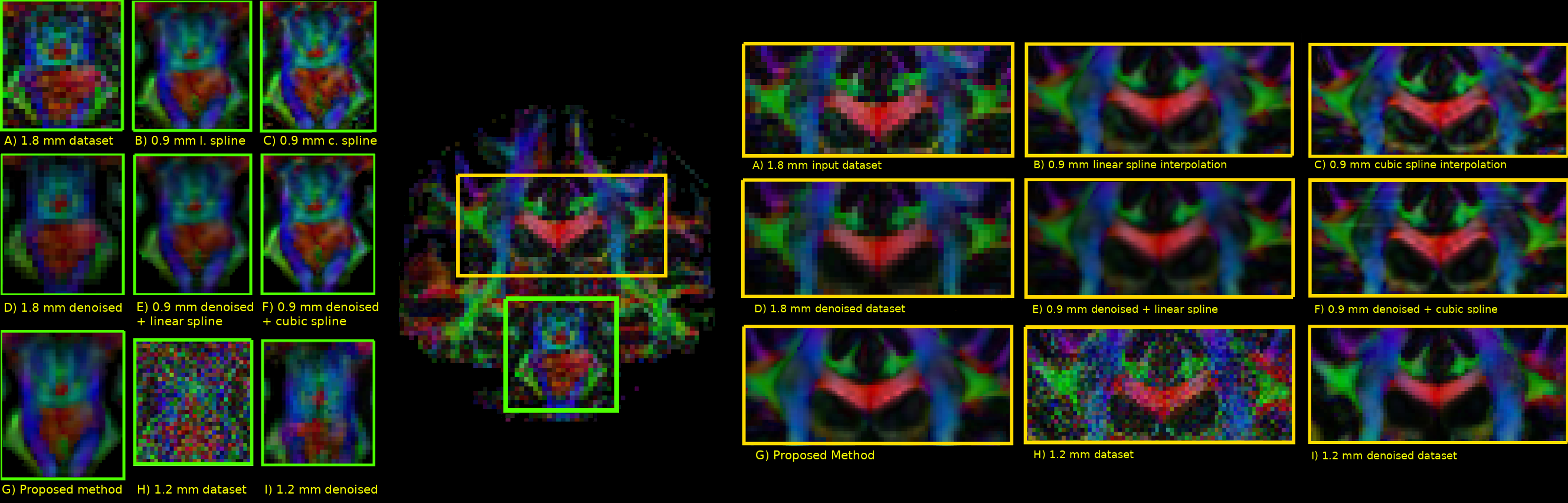
Figure 2 compares the raw data on the 1.8 mm dataset and the various upsampling on the original and denoised datasets on a coronal slice. The 1.2 mm dataset is also shown with its denoised version for anatomical comparison. Figure 3 shows two zoomed regions; the corpus callosum, the cingulum and the corticospinal tract and the pons region with the cerebellum. Figure 4 and 5 show the colored FA maps of the previous figures. Interpolation on the raw data leads to residual artefacts in the interpolated dataset. Applying denoising separately from interpolation introduces line artefacts or blurring, while our proposed combined approach preserves more details, but with the tradeoff of some blocking artefacts. Interpolation results are in agreement with the 1.2 mm raw and denoised dataset, even though they are produced from a 1.8 mm dataset.

Discussion and conclusion

We presented a new framework which combines two usually separate processing steps, namely denoising and upsampling, in a single unified framework. The proposed method links a set of lower and higher resolution patches, which permits reconstruction of dMRI data at a higher resolution than initially acquired without using specialized acquisition schemes. This category of approaches is particularly attractive since they can be applied on any already acquired datasets. As noted previously⁵, upsampling can reveal finer anatomical details which might help tractography, but care should be taken about possible biases or introduced artefacts in computed metrics such as FA. Moreover, our proposed method could be combined with acquisition techniques^1,2,3 to potentially improve the provided anatomical information.

Acknowledgements

Samuel St-Jean is supported by the Fonds de recherche du Québec – Nature et technologies (FRQNT). This research is supported by VIDI Grant 639.072.411 from the Netherlands Organisation for Scientific Research (NWO). Datasets were provided by the Centre d'imagerie moléculaire de Sherbrooke (CIMS) and the Sherbrooke Connectivity Imaging Lab (SCIL), Université de Sherbrooke, Sherbrooke, Québec, Canada.

References

1. Ning, L. et al., 2016. A joint compressed-sensing and super-resolution approach for very high-resolution diffusion imaging. NeuroImage

2. Scherrer, B. et al., 2015. Accelerated High Spatial Resolution Diffusion-Weighted Imaging. Information Processing in Medical Imaging

3. Van Steenkiste, G. et al., 2016. Super-resolution reconstruction of diffusion parameters from diffusion-weighted images with different slice orientations. Magnetic Resonance in Medicine

4. Coupé, P. et al., 2013. Collaborative patch-based super-resolution for diffusion-weighted images. NeuroImage

5. Dyrby, T.B. et al., 2014. Interpolation of diffusion weighted imaging datasets. NeuroImage

6. Yap, P.T. et al., 2014. Fiber-driven resolution enhancement of diffusion-weighted images. NeuroImage

7. Manjón, J. V. et al., 2010. Adaptive non-local means denoising of MR images with spatially varying noise levels. J. Magn. Reson. Imaging

8. St-Jean, S. et al., 2016. Non Local Spatial and Angular Matching : Enabling higher spatial resolution diffusion MRI datasets through adaptive denoising. Medical Image Analysis

9. Veraart, J. et al., 2016. Denoising of diffusion MRI using random matrix theory. NeuroImage

10. Rueda, A., et al., 2013. Single-image super-resolution of brain MR images using overcomplete dictionaries. Medical image analysis

11. Mairal, J. et al., 2009. Online Learning for Matrix Factorization and Sparse Coding. The Journal of Machine Learning

12. Glasner, D., et al. 2009. Super-Resolution from a Single Image. International Conference on Computer Vision (ICCV)

13. Koay, C.G., et al, 2009. Probabilistic Identification and Estimation of Noise (PIESNO): A self-consistent approach and its applications in MRI. Journal of Magnetic Resonance

14. Koay, C.G., et al., 2009. A signal transformational framework for breaking the noise floor and its applications in MRI. Journal of magnetic resonance

15. Tax, C. M.W., et al., 2015. REKINDLE: Robust extraction of kurtosis INDices with linear estimation. Magn. Reson. Med.

16. Leemans A. et al., 2009. ExploreDTI : a graphical toolbox for processing, analyzing, and visualizing diffusion MR data. 17th Annual Meeting of Intl. Soc. Mag. Reson. Med.

Figures

Figure 1: Schematic representation of the proposed framework. The dictionary $$$\textbf{D}$$$ is first computed with equation 1 and downsampled into $$$\textbf{d}$$$, which creates an exact mapping between the low and high resolution elements. $$$\alpha_i$$$ is then computed with equation 2 and $$$\textbf{d}$$$, which gives the final denoised and upsampled reconstruction using $$$\hat{X}_i=\textbf{D}\alpha_i$$$.

Figure 2: From left to right, top to bottom : A) the 1.8 mm input dataset B) linear spline interpolation of the 1.8 mm dataset C) cubic spline interpolation of the 1.8 mm dataset D) denoised version of the 1.8 mm dataset E) denoised, then linear spline interpolation F) denoised, then cubic spline interpolation G) the proposed method combining denoising and upsampling H) the 1.2 mm dataset I) the denoised 1.2 mm dataset. Interpolating the noisy data picks up most of the noise, while interpolating the denoised data is more blurry than our proposed framework.

Figure 3: A zoom of figure 2 showing the pons and the corpus callosum. In the pons, interpolation with or without denoising shows more blurring than the 1.2 mm denoised acquisition. Our proposed method can recover information which looks similar to the high resolution denoised acquisition. On the right, the contrast between the corpus callosum, the ventricules and the corticospinal tract is preserved with our proposed method, but is lost with the linear and cubic spline interpolation. The 1.2 mm dataset also has poor SNR in the ventricules, leading to diminished contrast after denoising.

Figure 4: A colored FA map of figure 2. Interpolation shows overall increased details, with the cubic spline picking up some ringing artefacts. On the denoised datasets, some line artefacts start to appear and are more common in the cubic spline interpolated version. In contrast, our proposed method does not seem to exhibit such issues, potentially due to the mapping between low and high resolution patches we employ which translates to local blocky artefacts instead. Nevertheless, our proposed method reconstruction is in agreement with the denoised 1.2 mm dataset, notably in the pons region.

Figure 5: A zoom of figure 4 showing the pons and the corpus callosum on a colored FA map. Spline interpolation picks up more details than the 1.8 mm dataset as seen by the green part coming out from the pons, but at the price of some artefacts for the linear version. Our proposed method shows nice delineation between the different structures, similar to the 1.2 mm denoised dataset. In the corpus callosum region, our proposed method keeps contrasts between the different bundles, but seem to pick up some ringing artefact near the ventricules.

Proc. Intl. Soc. Mag. Reson. Med. 25 (2017)

3533