3523
Transfer learning and convolutional neural net fusion for motion artefact detection1Centre for the Developing Brain, King's College London, London, United Kingdom
Synopsis
The first step in a diffusion MRI pre-processing pipeline typically involves the manual removal of heavily motion-corrupted volumes. However, this process is both time consuming and potentially subjective. We propose to automate this process by training multiple deep convolutional neural networks (CNNs) and decision trees to achieve near human-level accuracy for rejection of outliers.
Introduction
The first step in a pre-processing pipeline for diffusion MRI typically involves manually removing motion-artefacted volumes, particularly in neonates. This process is both time-consuming and potentially subjective. Existing tools for outlier detection and replacement perform well in volumes with motion artefacts in isolated slices, but relatively poorly in cases with severe motion that affect the whole volume. It is therefore common practice to remove such volumes manually before proceeding with the usual pipeline. We propose a solution based on computer vision techniques to automate the current manual review process with human levels of performance.Methods
Diffusion weighted volumes for 36 term neonatal subjects were acquired in natural sleep, using a 3T Philips Achieva MR scanner with dedicated 32-channel neonatal head coil and patient handling system1, situated on the neonatal intensive care unit at St Thomas’ Hospital, London. A highly optimized neonatal diffusion sequence was used (4 phase encode (PE) directions, b = 0, 400, 1000 and 2600s/mm2, 1.5x1.5x3mm voxels)2.
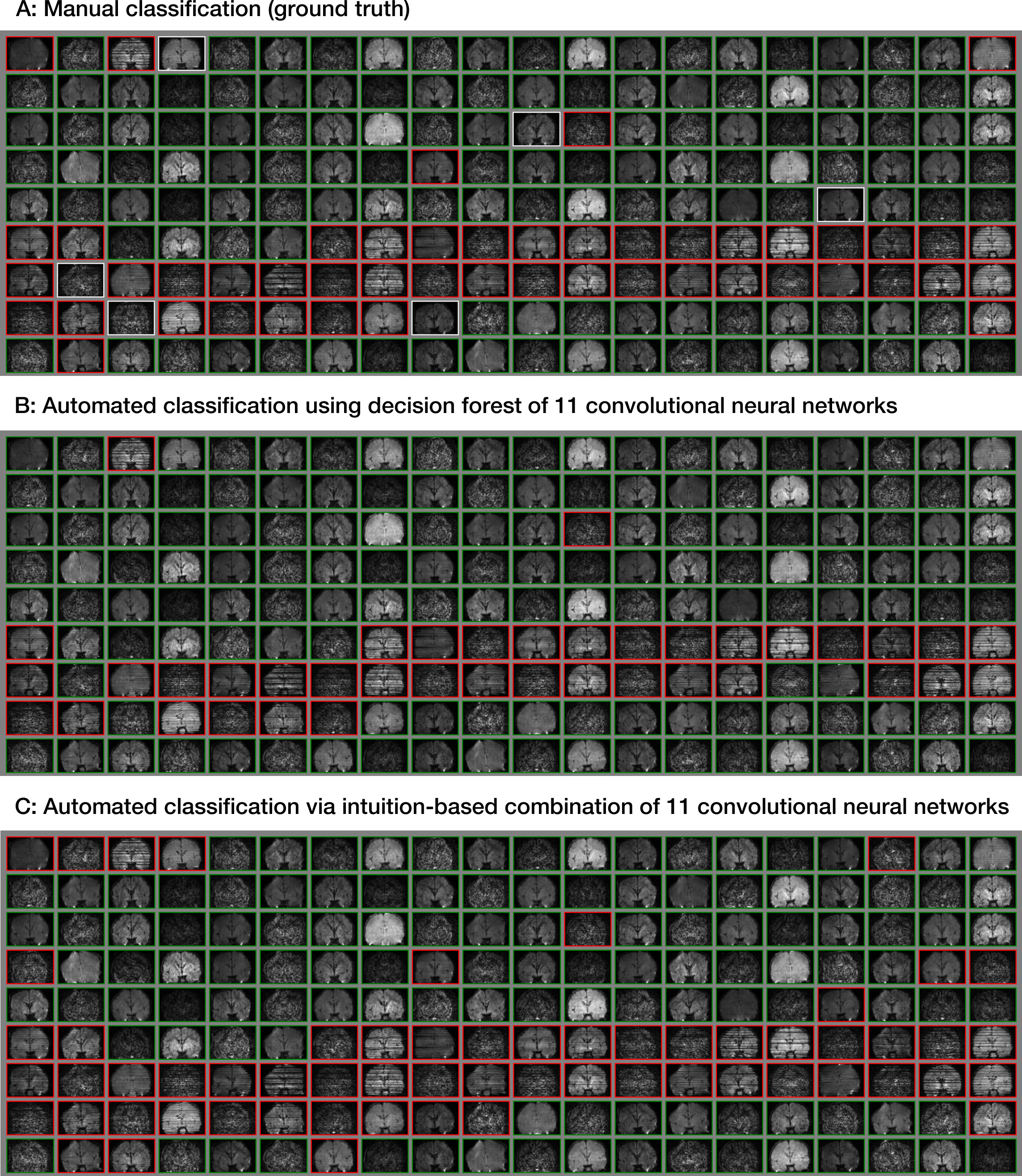
Volumes were annotated manually by visual inspection into three categories: accept, borderline, and reject. 2D slices were extracted from all 300 diffusion-weighted volumes for each subject in three orientations, through the center of gravity and six adjacent parallel planes, resulting in a dataset containing 207,249 labelled images.
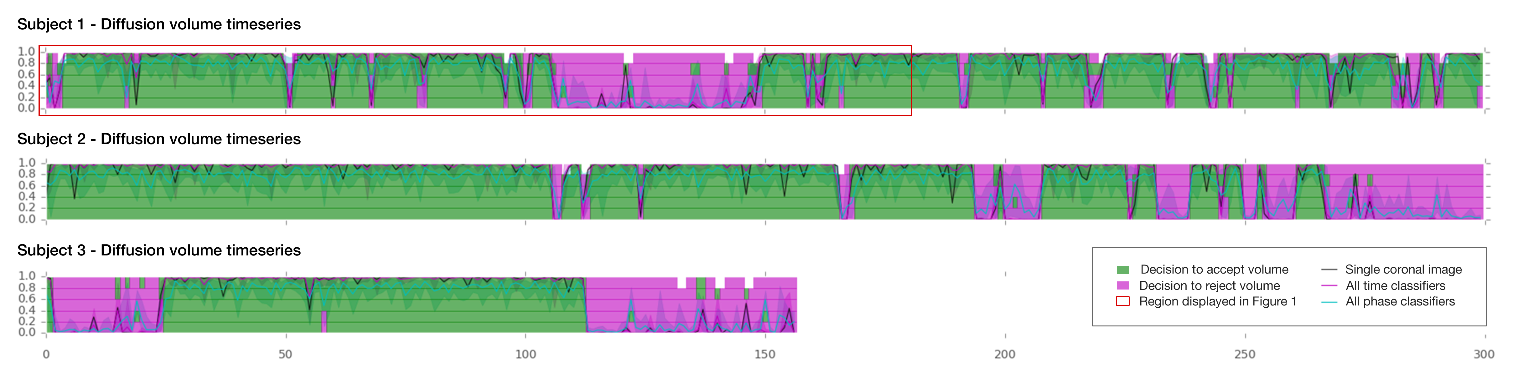
We used a convolutional neural network (CNN) design called InceptionV33, which has previously been pre-trained on 1,000,000 general purpose images. Using the Tensorflow framework4, we retrained 11 new distinct top layers from different aspects of the data: 6 DWI magnitude layers (b0, b400, b1000, b2600, all b-values, agnostic to b-value) and 5 phase image layers (b400, b1000, b2500, all b-values, agnostic to b-value). Borderline cases were ignored for the CNN training and accuracy testing. The training data for each subject consisted of multiple sagittal and coronal slices for the magnitude image classification or multiple axial slices for the phase image classification. To integrate all CNN outputs, a forest of up to 600 decision trees was trained on 7 subjects using a binary adaptive boosting algorithm. The accuracy to predict “accept” labels was tested on 1072 volumes from four subjects.
This two-step approach allows the ability to retrospectively change the image classification criteria by manually thresholding the CNN final layer output (softmax), avoiding the need to relabel the ground truth or retrain the CNN.
An “intuition-based” approach was also implemented based on the following rule: if mean reject probability for magnitude and phase image > 0.5, or mean magnitude reject probability > 0.85.
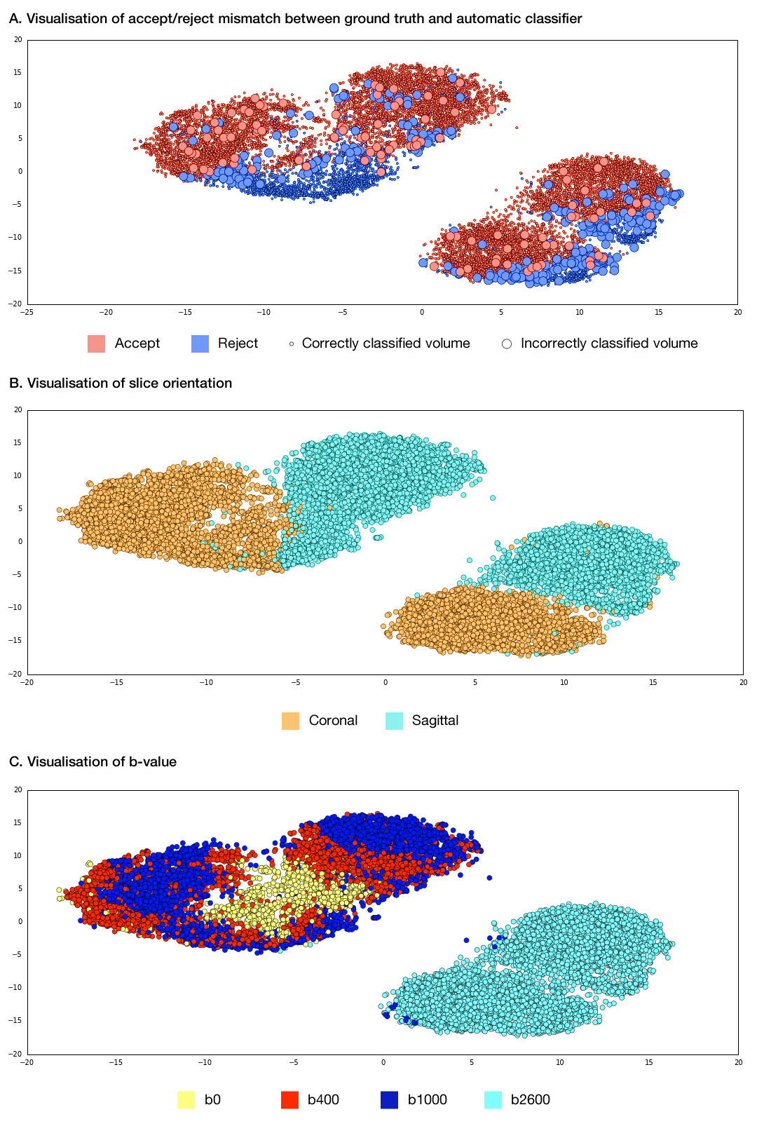
Results were visualised via PCA and t-Distributed Stochastic Neighbor Embedding (t-SNE)5, which is a dimensionality reduction technique that preserves local structure.
Results
The best individual CNN achieved accuracies when labelling accept/reject between 96.8% and 98% in each diffusion weighting category, while the average of the individual classifier accuracies varied between 86.6% and 93.4%. The decision tree forest yielded accuracies of 94.8% - 99.4% and assigned weights that identified the majority of model features as important. Examples of classification of individual volumes can be seen in Figure 1, which have been derived from the individual components of the model as demonstrated in Figure 2.
For comparison, intraobserver and interobserver accuracy for two observers performing the same classification task on 1200 volumes was 99.2% and 99.3% respectively, excluding borderline labels. Including borderline labels resulted in intraobserver and interobserver accuracy of 95.4% and 88.7%, respectively.
t-SNE plots (Figure 3) show that the volumes are well-segmented by the model, with borderline cases (plot A) generally occurring at the borderline between accept and reject.
Discussion
A convolutional neural network approach to detect motion artefacts in diffusion MRI data can demonstrate human-level accuracy in a task that has historically been difficult to automate. t-SNE visualization shows borderline cases are generally at the interface between accept and reject clusters, supporting the validity of the method.Conclusion
This technique can be implemented as a first step in a pre-processing pipeline for neonatal diffusion datasets, avoiding the need for time-consuming manual exclusion of heavily motion-corrupted datasets. Insights from graphs generated automatically by this approach may facilitate the creation of new tools for quality assurance and artefact detection.Acknowledgements
MRC strategic funds (MR/K006355/1), British Heart Foundation Clinical Research Training Fellowship (FS/15/55/31649), and the GSTT BRC.References
1. Hughes, E. J. et al. A dedicated neonatal brain imaging system. Magn Reson Med (2016).
2. Tournier, J. D. et al. Data-driven optimisation of multi-shell HARDI in Annual meeting of the ISMRM. Toronto, Canada (2015).
3. Szegedy C, Vanhoucke V, Ioffe S, Shlens J, Wojna Z (2015), Rethinking the Inception Architecture for Computer Vision, https://arxiv.org/abs/1512.00567
4. Abadi, M et al (2015), TensorFlow: Large-scale machine learning on heterogeneous systems, http://download.tensorflow.org/paper/whitepaper2015.pdf
5. van der Maaten L, Hinton G. Visualizing Data using t-SNE, Journal of Machine Learning Research 9 (2008) 2579-2605.
Figures