3508
Free-water elimination in diffusion MRI: pushing the limits towards clinical applications1Institute of Neuroscience and Medicine 4, Forschungszentrum Jülich, Jülich, Germany, 2Department of Neurology, Faculty of Medicine, RWTH Aachen University, Aachen, Germany, 3JARA – BRAIN – Translational Medicine, RWTH Aachen University, Aachen, Germany
Synopsis
Free-water elimination allows one to reduce the bias in DTI metrics induced by partial-volume effects. In this work, we propose a versatile approach for the optimisation of the diffusion weighting settings, given a limited acquisition time, based on a parameterised Cramér-Rao lower-bound. The optimisation shows robust convergence.
Purpose
Free-water elimination (FWE) has been proposed to reduce the bias in DTI metrics induced by partial-volume effects.1,2,3 It has been recently shown to be sensitive to the free-water content in the substantia nigra in Parkinson’s patients.4,5 In the quest of performing FWE DTI under clinically feasible conditions, an optimised protocol, such that the variances of the parameters of interest are minimised, is desired. The optimisation of diffusion weighting (DW) settings for FWE DTI has been previously proposed6, based on model simulations. Here, we approach the problem from a different, more versatile perspective, which allows one to systematically obtain the optimal protocol given a maximum acquisition time. We optimise the DW settings via minimisation of the Cramér-Rao lower-bound (CRLB)7,8,9 of a set of parameters of interest.Methods
FWE DTI. The model we adopt here assumes that the normalised, diffusion MRI signal originates from two compartments in the slow-exchange limit1,2:
$$S\left(b,\mathbf{g},\boldsymbol{\theta}\right)=f_\mathrm{w}\mathrm{exp}\left(-bD_0\right) + \left(1-f_\text{w}\right)\mathrm{exp}\left(-b\mathbf{g}^T\mathbf{Dg}\right)\text{,}$$
where $$$f_\mathrm{w}$$$ and $$$D_0$$$ are the fraction and the diffusion coefficient of the free-water compartment, respectively, $$$\mathbf{D}$$$ is the diffusion tensor for the tissue compartment, $$$\boldsymbol{\theta}\equiv\left(f_\mathrm{w},D_{11},D_{12},D_{13},D_{22},D_{23},D_{33}\right)$$$ and b and g are the strength and direction of the DW gradient, respectively. D0=3μm2/ms is fixed1,2 to the diffusion coefficient of free water at 37ºC.
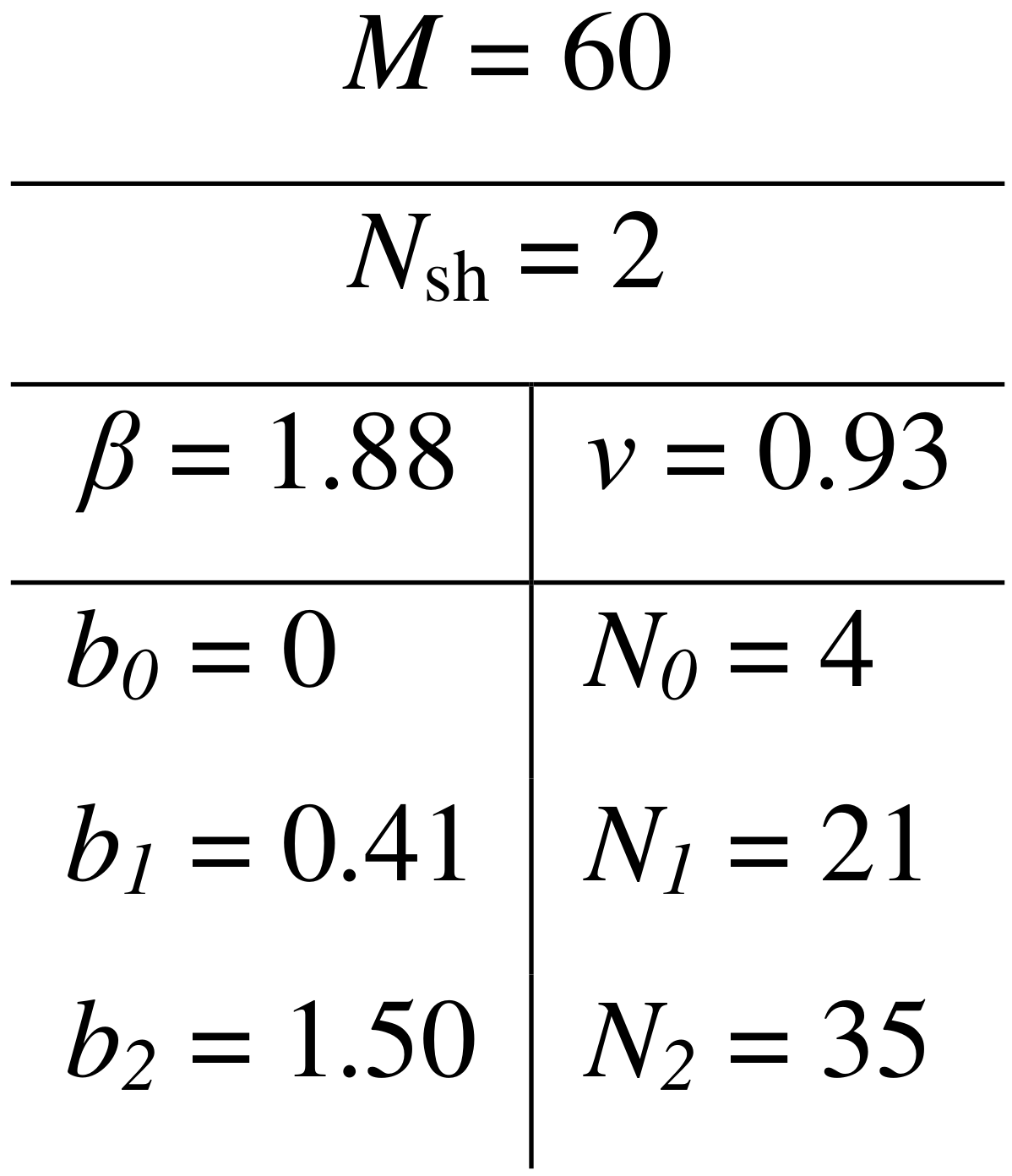
Parameterisation. The DW settings are parameterised following Ref.9 They consist of $$$N_\mathrm{sh}$$$ shells, with the $$$i^{th}$$$ shell having a radius $$$b_i$$$ and containing $$$N_i$$$ isotropically distributed10 gradient directions ($$$i=0...N_\mathrm{sh}$$$). The distributions for $$$b_i$$$ and $$$N_i$$$ are given by: $$$b_i=b_\mathrm{max}\eta_i^\beta$$$ and $$$N_i=N_0+\left(N_\mathrm{max}-N_0\right)\eta_i^\nu$$$, where $$$\eta_i=i/N_\mathrm{sh}$$$, $$$b_\mathrm{max}$$$ is the maximum b-value, $$$N_0$$$ is the number of non-diffusion-weighted volumes and $$$N_\mathrm{max}$$$ is the number of gradient directions at the outermost shell (determined by the total amount of volumes $$$M$$$). Thus, the DW settings are completely determined by the vector $$$\mathbf{P}=\left(M,N_\mathrm{sh},N_0,\boldsymbol{\beta},\boldsymbol{\nu},b_\mathrm{max}\right)$$$. In order to account for SNR reductions due to gradient strength limitations for increasing b-values, we parameterise the SNR following Ref.7
Optimisation. The optimal $$$\mathbf{P}$$$ is found by simultaneously minimising the CRLB of $$$f_\mathrm{w}$$$ and $$$D_{i,j}$$$ ($$$i,j$$$=1,2,3)8,9. The objective function to be minimised is9:
$$H\left[\mathbf{P},\rho\right]=\sum_{k=1}^{T}\rho_k\|\boldsymbol{\Omega}\left(\boldsymbol{\theta_k}\right)\|_2\text{,}$$
where $$$\rho_k$$$ ($$$k=1...T$$$ spans the number of tissue types8,9) is the probability for the k-th tissue with diffusion properties $$$\boldsymbol{\theta}_k$$$ . Here we take $$$T=2$$$, i.e., grey and white matter. The elements of the vector $$$\boldsymbol{\Omega}$$$, $$$\Omega_l\equiv\sqrt{I_l^{-1}}$$$ , contain the CRLB, $$$I_l^{-1}$$$, of the parameters $$$\theta_l$$$ ($$$l=1,...,7$$$). The performance of two algorithms for the minimisation of $$$H$$$ was carried out and compared:
Algorithm 1: the local, computationally simple Nelder-Mead algorithm.
Algorithm 2: the global, computationally expensive genetic algorithm, both available in Matlab (Matlab, The MathWorks).
The upper constraint for $$$b_\mathrm{max}$$$ was set to 1.5 ms/μm2 in order to avoid non-Gaussian effects6.
In vivo experiments. Experiments were performed on a healthy volunteer, in a 3T Trio scanner (Siemens Erlangen, Germany) using the twice-refocused bipolar spin-echo EPI pulse sequence. The optimised DW settings for an acquisition time of 8:30 minutes are shown in Table 1. Other protocol parameters were: TR=8100ms; TE=94ms; voxel-size=2×2×2mm3; BW=1446Hz/pixel; matrix-size128×128×60; GRAPPA accel. factor=2.
Data analysis. Eddy current and EPI distortions were corrected using the EDDY toolkit available in FSL11. FWE DTI parameter estimation was performed in two steps:
i) an initial guess for the tensor elements was generated by fitting conventional DTI;
ii) FWE DTI was fitted via non-linear least-squares minimisation using the initial guess generated in step i), with the help of the Levenberg-Marquardt algorithm with in-house Matlab scripts.
Results and discussions
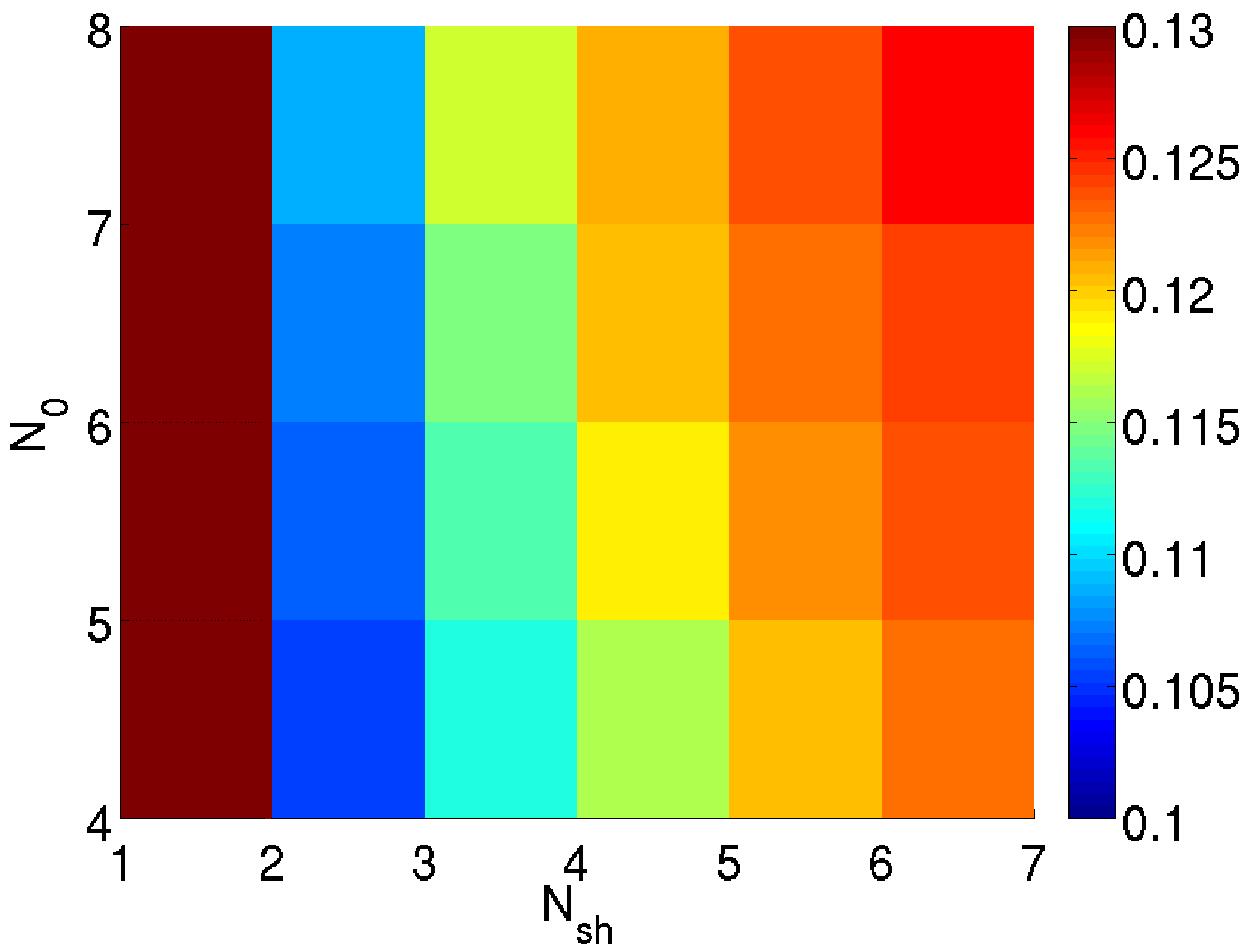
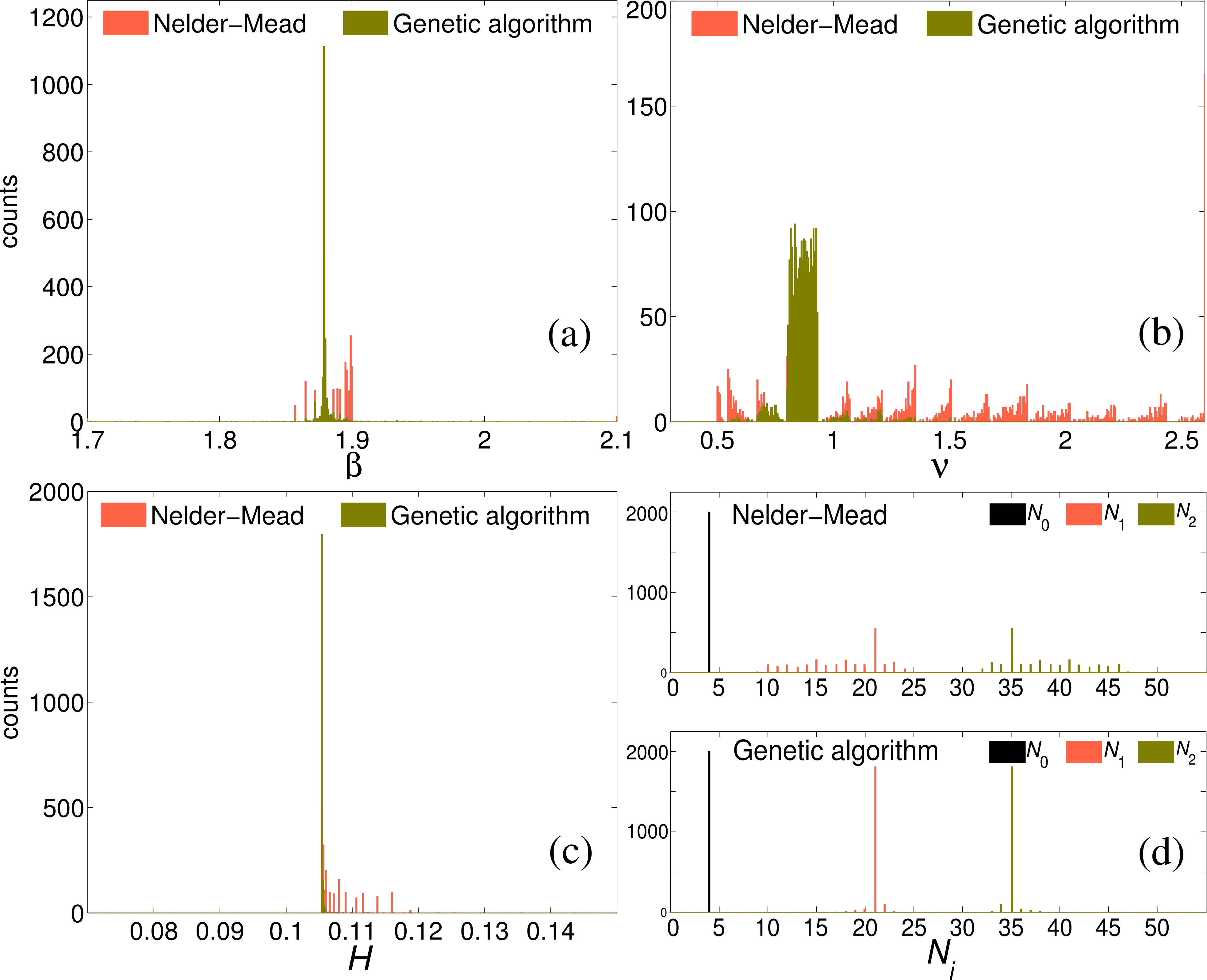
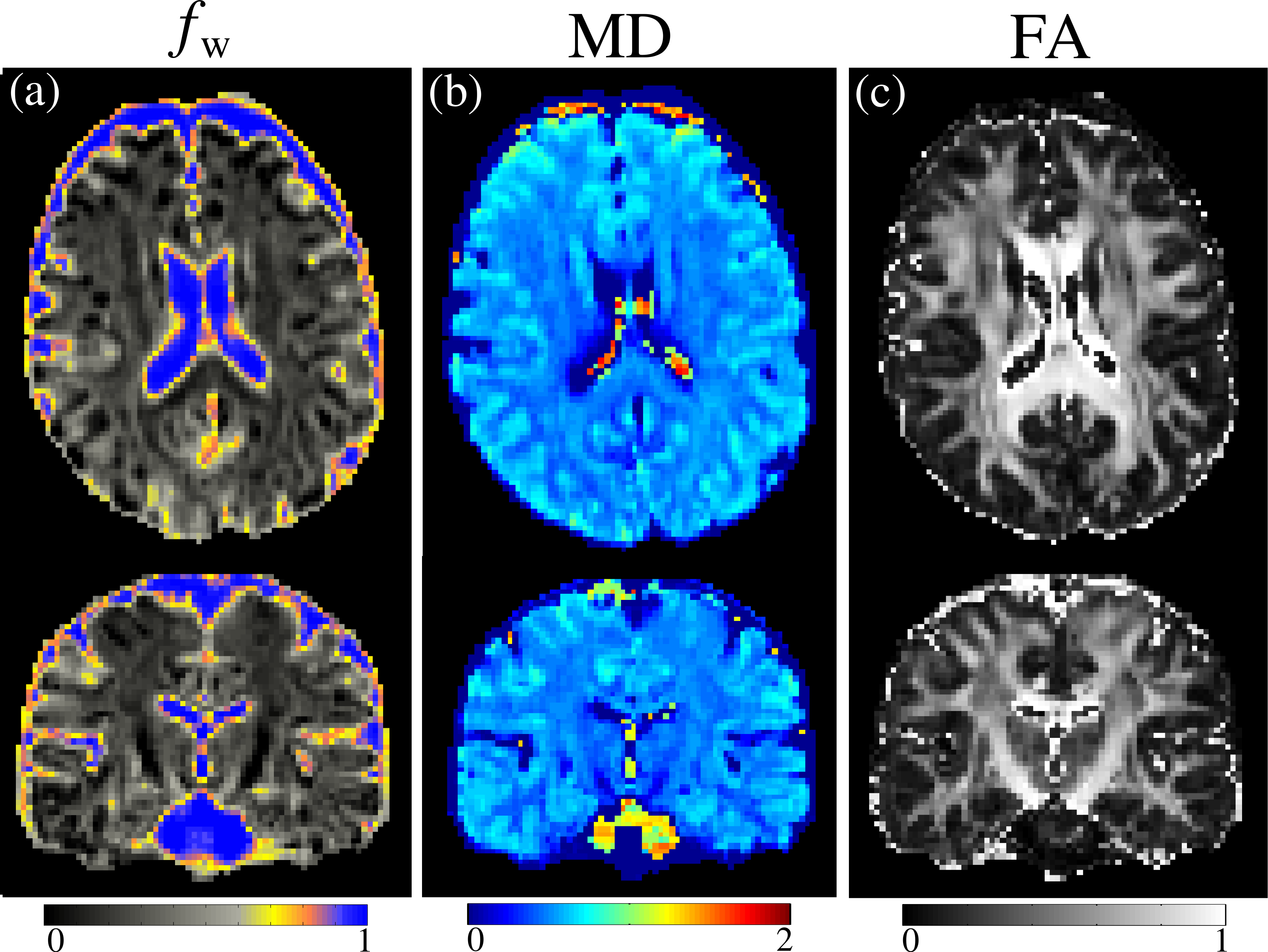
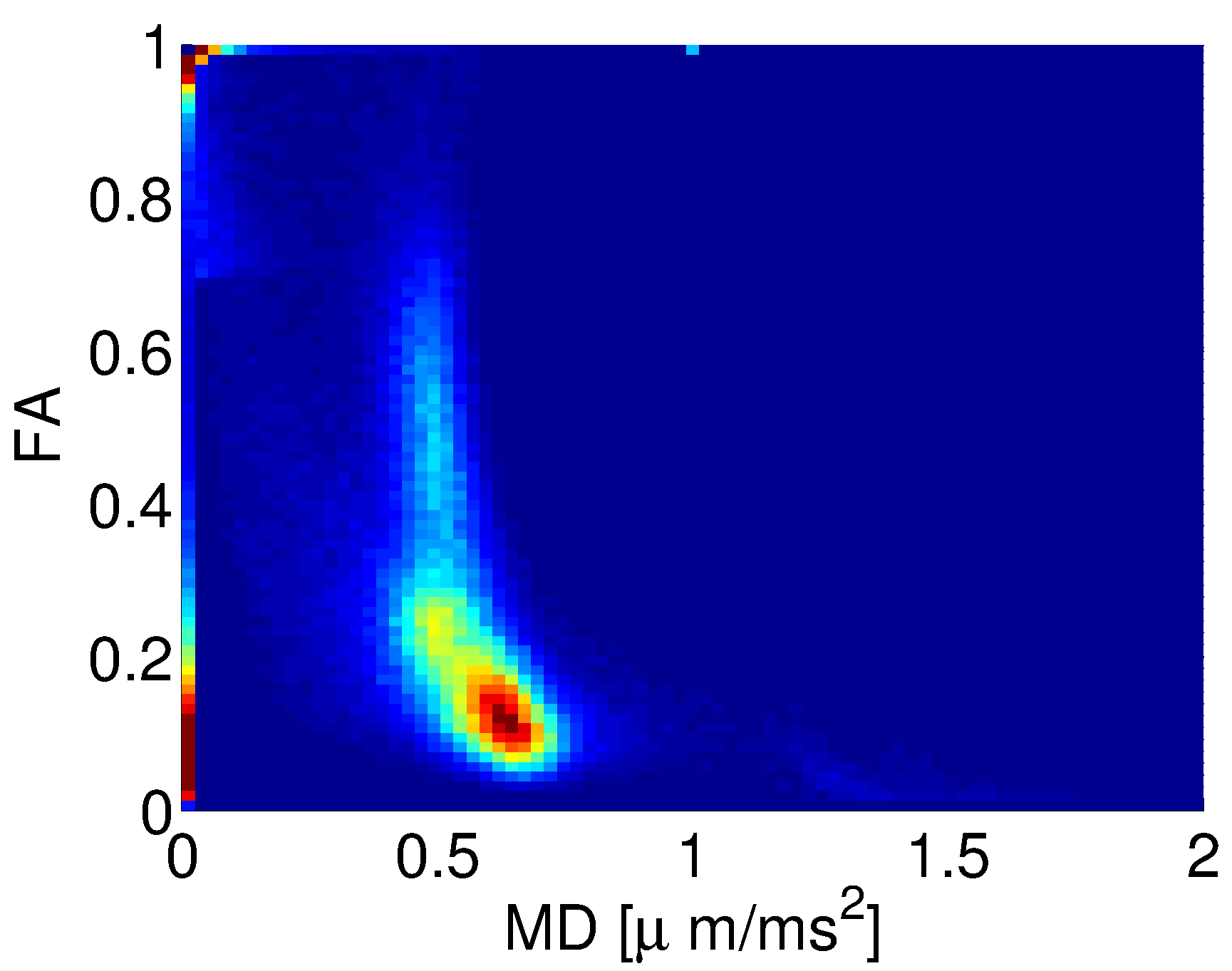
Figure 1 shows the minimised values of $$$H$$$ vs. $$$N_\mathrm{sh}$$$ and $$$N_0$$$. The optimal number of shells is clearly $$$N_\mathrm{sh}=2$$$. For $$$N_\mathrm{sh}=2$$$, there is an increase of $$$H$$$ with increasing $$$N_0$$$. Here we take $$$N_0=4$$$ interspersed with the diffusion-weighted volumes. Figure 2 shows the distribution of the optimal parameters, upon 2000 random initialisations for each algorithm. The Nelder-Mead algorithm clearly presents convergence problems. On the other hand, one can observe a unimodal parameter distribution for the genetic algorithm. This shows that the cost function $$$H$$$ is globally convex. Optimal parameters are shown in Table 1. Figure 3 shows the maps of $$$f_\mathrm{w}$$$, mean diffusivity (MD), and fractional anisotropy (FA) for the tissue compartment. Figure 4 shows the joint histogram of FA vs. MD. One can see that the use of FWE DTI allows one to evaluate the only-tissue diffusion characteristics6.Conclusions
We have successfully adapted a previously proposed approach9 for the optimisation of the DW settings in the framework of FWE DTI. The optimisation shows robust convergence using the genetic algorithm. It allows one to systematically design optimal DW settings for a desired acquisition time.Acknowledgements
No acknowledgement found.References
1. Pasternak, O., et al. Magn. Reson. Med. 2009; 62:717-730;
2. Pasternak, O., et al. Med Image Comput Comput Assist Interv. 2012; 15:305-312;
3. Caan, M.W.A., et al. IEEE TMI 2010; 29:1504-1515;
4. Ofori, E., et al. Neurobiol Aging. 2015; 36:1097–1104;
5. Ofori, E., et al. Brain. 2015; 138:2322-2331;
6. Hoy, A.R., et al. Neuroimage 2014; 103:323–333;
7. Alexander, C.A. Magn. Reson. Med. 2008; 60:439-448;
8. Poot, D.H.J., et al. IEEE 2010; 29:819-829;
9. Farrher, E., et a. Proc. Intl. Soc. Mag. Reson. Med. 2016; 24:3018;
10. Stirnberg, R., et al. Proc. Intl. Soc. Mag. Reson. Med. 2009; 17:3574;
11. Andersson, J.L.R., and Sotiropoulos, S.N. NeuroImage 2016, 125:1063-1078.
Figures