3493
Exponential Decay Law for the Structural Brain Network of Maltreated Children1Waksman Laboratory for Brain Imaging and Behavior, University of Wisconsin, Madison, WI, United States, 2Department of Psychology, University of Pittsburgh, Pittsburgh, PA, United States, 3Department of Psychology, University of Wisconsin, Madison, WI, United States
Synopsis
We present evidence that the structural brain network follows the exponential decay law; these data are inconsistent with the view the brain follows the more complicated truncated exponential power law. Our model is then used in application, to show that children exposed to high levels of early life stress have more sparsely connected hub nodes. These data are consistent with rodent models of the effects of stress on synaptogenesis.
Introduction
Node degree is one of the most widely used network features. The precise determination of the degree distribution is critical for many applications. Previous studies have shown that the human brain network is not scale-free and does not follow the power law1,2,3. Hagmann1 reported that degree decayed exponentially while Gong2 reported the degree decayed in an exponentially truncated power law. In this study, we show that the structural brain network follows the exponential decay law using a more robust estimation technique. The estimated model is then used to quantify that maltreated children have less dense connections in major hub nodes.Methods
Data: The study consisted of 23 children who experienced maltreatment early in their lives, and 31 age-matched normal controls. The maltreated children were raised in institutional settings, where the quality of care has been below the standard necessary for healthy development. The age distribution is 11.44±1.64 years. The average amount of time spent in institutional care range from 3 months to 5.4 years. Children were on average 3.2 years when they were adopted, with a range of 3 months to 7.7 years. DTI were collected on a 3T GE SIGNA scanner. Diffusion tensor encoding was achieved using 12 optimum non-collinear encoding directions with a diffusion weighting of 1114 s/mm2. The details on acquisition parameters are given in Hanson4.
Processing: DTI processing follows the pipeline established in the previous studies4,5,6,7. Spatial normalization of DTI data was done using diffeomorphic registration5. Tractography was done using the TEND algorithm7. Anatomical Automatic Labeling (AAL) with 116 parcellations were used to establish network nodes8. The tracts counts were used in building adjacency matrices.
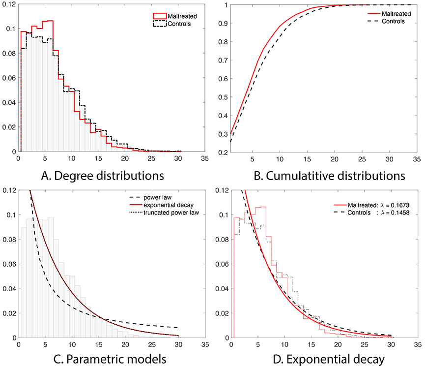
Degree distributions: The node degree $$$k$$$, which counts the number of connections at the node, was measured. The two-sample t-test on the node degree did not yield any group difference (Figure-1). It was necessary to use a more sophisticated approach. The previous studies reported the probability distribution $$$P(k)$$$ to follow one of three laws1,2,3:
Power law: $$ P_{p}(k){\sim}k^{-\gamma},$$
Exponential decay: $$P_{e}(k){\sim}e^{-\lambda{k}},$$
Exponentially truncated power law: $$P_{etp}(k){\sim}k^{-\gamma}e^{-\lambda k}.$$ Estimating the parameters from the empirical distribution is challenging due to small sample size in the tail region. The parameters were estimated from the cumulative distribution functions (CDF) that accumulate the probability from low to high degrees to reduces noise in the tail region. We further combined all the degrees across the subjects to increase the sample size further. The parameters were estimated by minimizing the sum of squared errors (SSE) between the theoretical and empirical CDFs. For instance, in the exponentially truncated power law $$(\widehat\gamma,\widehat\lambda)=\arg\min_{\gamma\geq0,\lambda\geq0} \int_{0}^{\infty}\big| F_{etp}(k)-\widehat{F}_{etp}(k)\big|_2^2\;dk.$$
Results
Exponential decay: The best model was for the power law was when γ=0.2794 with SSE=1.01. For the exponential decay law, the best model was when λ=0.1500 with SSE=0.046. For the truncated power law, the best model was when γ=0,λ=0.1500 with SSE=0.046. The best truncated power law became the exponential decay when γ=0. Thus, our data supports the exponential decay model (Figure-2).
The maltreated subjects had higher concentration in low degree nodes. The controls had much higher concentration of hub nodes. This pattern is also observed in the cumulative distribution functions (CDF) for each group. The maltreated subjects clearly show higher cumulative probability at lower degree.
Group comparisons: Once we determined the degree distribution follows the exponential decay model for all 54 subjects, we fitted the exponential decay model for each subject separately to see if there is any group difference in the estimated parameter. The estimated parameters were 0.1673±0.0341 for the maltreated children and 0.1458±0.0314 for the controls. The controls showed a slightly heavier tail compared to that of the maltreated children. The two-sample t-test was performed on the parameter difference obtaining significant result (t-stat.=2.40, p-value<0.02). The controls had a higher concentration of hub nodes.
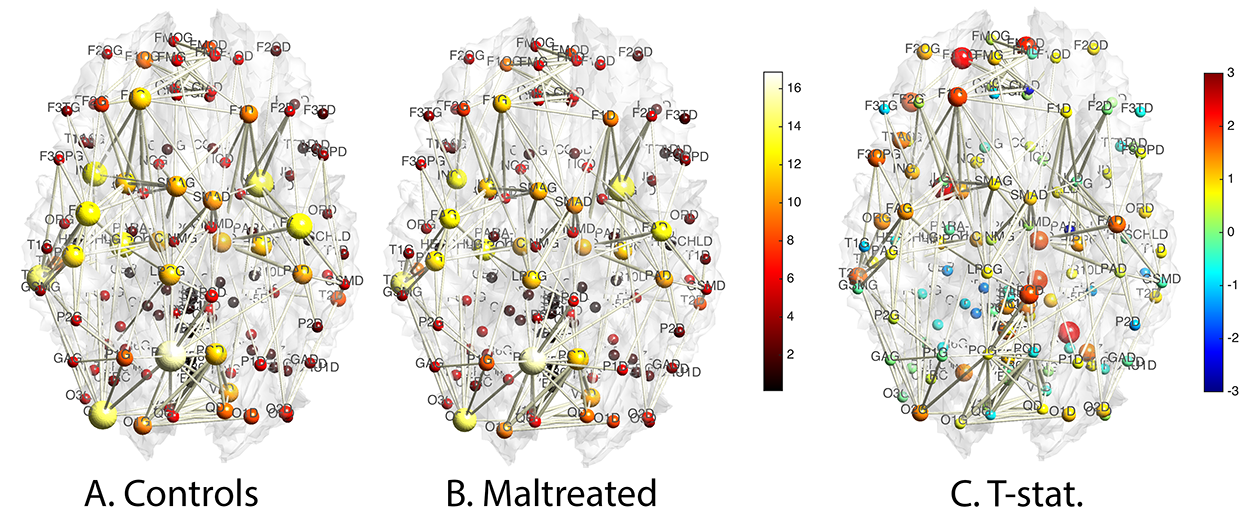
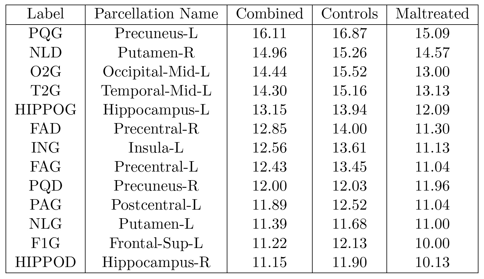
Hub nodes: We determined the 13 most connected nodes (Figure-3), all of which showed higher numbers of connections. The probability of this outcome occurring by a chance is 2-13=0.00012. Thus, the controls are more highly connected in the hub nodes compared to the maltreated children.
Conclusions
Less connected hub nodes after maltreatment were found in the putamen, hippocampus, precuneus, and portions of the prefrontal cortex. This fits with alterations in emotion and reward processing seen after stress exposure. The hippocampus and superior frontal gyrus have been implicated in aspects of emotion regulation, while the putamen is involved with understanding rewards in the environment. Fewer less dense network nodes may make it harder for children who have suffered stress to integrate incoming information from the environment and process these signals.Acknowledgements
This work was supported by NIH Grants MH61285, MH68858, MH84051, UL1TR000427 and EB022856.References
[1] G. Gong, Y. He, L. Concha, C. Lebel, D. W. Gross, A. C. Evans, and C. Beaulieu. Mapping anatomical connectivity patterns of human cerebral cortex using in vivo diffusion tensor imaging tractography. Cerebral cortex, 19:524–536, 2009.
[2] P. Hagmann, L. Cammoun, X. Gigandet, R. Meuli, C. Honey, V. J. Wedeen, and O. Sporns. Mapping the structural core of human cerebral cortex. PLoS Biolology, 6 (7):e159, 2008.
[3] A. Zalesky, A. Fornito, I. Harding, L. Cocchi, M. Yücel, C. Pantelis, and E. Bullmore. Whole-brain anatomical networks: Does the choice of nodes matter? NeuroImage, 50: 970–983, 2010.
[4] J. Hanson, N. Adluru, M. Chung, A. Alexander, R. Davidson, and S. Pollak. 2013 Early neglect is associated with alterations in white matter integrity and cognitive functioning. Child Development, 84:1566–1578, 2013.
[5] H. Zhang, B. Avants, P. Yushkevich, J. Woo, S. Wang, L. McCluskey, L. Elman, E. Mel- hem, and J. Gee. High-dimensional spatial normalization of diffusion tensor images improves the detection of white matter differences: An example study using amyotrophic lateral sclerosis. IEEE Transactions on Medical Imaging, 26:1585–1597, 2007.
[6] Chung, M.K., Adluru, N., Dalton, K.M., Alexander, A.L., Davidson, R.J. 2011. Scalable brain network construction on white matter fibers. Proceedings of SPIE. 7962, 79624G.
[7] M. Lazar, D. Weinstein, J. Tsuruda, K. Hasan, K. Arfanakis, M. Meyerand, B. Badie, H. Rowley, V. Haughton, A. Field, B. Witwer, and A. Alexander. White matter tractography using tensor deflection. Human Brain Mapping, 18:306–321, 2003.
[8] N. Tzourio-Mazoyer, B. Landeau, D. Papathanassiou, F. Crivello, O. Etard, N. Delcroix, B. Mazoyer, and M. Joliot. Automated anatomical labeling of activations in spm using a macroscopic anatomical parcellation of the MNI MRI single-subject brain. NeuroImage, 15:273–289, 2002.
Figures