Synopsis

Construction of brain atlases is generally carried out using a two-step procedure involving registering a population of images to a common space and then fusing the aligned images to form an atlas. In practice, image registration is not perfect and simple averaging of the images will blur structures and cause artifacts. In diffusion MRI, the problem is even more challenging, since the alignment of gross anatomical structures does not necessarily guarantee the alignment of the microstructural information captured in each voxel. In this situation, it is unclear for example how signals characterizing fiber bundles of varying orientations, which can occur naturally across subjects, should be fused to form the atlas. Moreover, the commonly used simple averaging method is sensitive to outliers.

Method

Our method employs neighborhood matching in $$$q$$$-space for effective atlas construction. See Fig. 1 for an overview. For each point in the $$$x$$$-$$$q$$$ space, $$$(\mathbf{x}_{i},\mathbf{q}_{k})$$$, where $$$\mathbf{x}_{i}\in\mathbb{R}^3$$$ is a voxel location and $$$\mathbf{q}_{k}\in\mathbb{R}^{3}$$$ is a wavevector, we define a spherical patch, $$$\mathcal{P}_{i,k}$$$, centered at $$$\mathbf{q}_{k}$$$ with fixed $$$q_{k} = | \mathbf{q}_{k} |$$$ and subject to a neighborhood angle $$$\alpha_{p}$$$. The diffusion measurements on this spherical patch is mapped to a disc using azimuthal equidistant projection (AEP)¹ before computing the rotation invariant features via polar complex exponential transform (PCET)² for patch matching. PCET with order $$$n$$$, $$$|n|=0,1,2,\dots,\infty$$$, and repetition $$$l$$$, $$$|l|=0,1,2,\dots,\infty$$$, of AEP-projected signal profile $$${S}(\mathbf{x},q,\rho,\theta)$$$ is defined as \begin{equation}\label{eq:pcet} M_{n,l}(\widehat{\mathcal{P}})=\frac{1}{\pi}\int_{(\mathbf{x},q,\rho,\theta)\in{\widehat{\mathcal{P}}}}[H_{n,l}(\rho,\theta)]^{*}{S}(\mathbf{x},q,\rho,\theta)\rho\operatorname{d}\rho\operatorname{d}\theta, \end{equation} where $$$[\cdot]^{*}$$$ denotes the complex conjugate and $$$H_{n,l}(\rho,\theta)$$$ is the basis function defined as\begin{equation}H_{n,l}(\rho,\theta)=e^{i2\pi{nr^{2}}}e^{il\theta},\end{equation}For each patch $$$\widehat{\mathcal{P}}$$$ consisting of signal vector $$$\mathbf{S}(\widehat{\mathcal{P}})$$$, the associated PCET features $$$\{|M_{n,l}(\widehat{\mathcal{P}})|\}$$$ computed up to maximum order $$$m$$$ (i.e., $$$0 \leq l, n \leq m$$$) are concatenated into a feature vector $$$\mathbf{M}(\widehat{\mathcal{P}})$$$.

The similarity of a reference patch $$$\widehat{\mathcal{P}}_{i,k}$$$ with another patch $$$\widehat{\mathcal{P}}_{j,l}(d)$$$ associated with the $$$d$$$-th subject is characterized by weight\begin{equation}\label{eq:weight}w_{i,k;j,l}=\frac{1}{Z_{i,k}}\exp\left\{-\frac{\|\mathbf{M}({\widehat{\mathcal{P}}}_{i,k})-\mathbf{M}({\widehat{\mathcal{P}}}_{j,l})\|^{2}_{2}}{h^{2}_{\mathbf{M}}(i,k)}\right\}\exp\left\{-\frac{\|\mathbf{x}_{i}-\mathbf{x}_{j}\|^{2}_{2}}{h^{2}_{\mathbf{x}}}\right\},\end{equation}where $$$Z_{i,k}$$$ is a normalization constant to ensure that the weights sum to one, i.e.,\begin{equation}Z_{i,k}=\sum_{(\mathbf{x}_{j},\mathbf{q}_{l})\in\mathcal{V}_{i,k}}\exp\left\{-\frac{\|\mathbf{M}(\widehat{\mathcal{P}}_{i,k})-\mathbf{M}(\widehat{\mathcal{P}}_{j,l})\|^{2}_{2}}{h^{2}_{\mathbf{M}}(i,k)}\right\}\exp\left\{-\frac{\|\mathbf{x}_{i}-\mathbf{x}_{j}\|^{2}_{2}}{h^{2}_{\mathbf{x}}}\right\}.\end{equation}Here $$$h_{\mathbf{M}}(i,k)$$$ is a parameter controlling the attenuation of the exponential function. As in Coupé's paper³, we set $$$h_{\mathbf{M}}(i,k)=\sqrt{2\beta\hat{\sigma}_{i,k}^{2}|\mathbf{M}(\widehat{\mathcal{P}}_{i,k})|}$$$, where $$$\beta$$$ is a constant, $$$\hat{\sigma}_{i,k}^{2}$$$ is the estimated noise standard deviation, which can be computed globally⁴ or spatial-adaptively³. The former is used in this paper. Parameter $$$h_{\mathbf{x}}=\sqrt{2}\sigma_{\mathbf{x}}$$$ controls the attenuation of the second exponential function, where $$$\sigma_{\mathbf{x}}$$$ is a scale parameter. $$$|\mathbf{M}(\widehat{\mathcal{P}}_{i,k})|$$$ denotes the length of the vector $$$\mathbf{M}(\widehat{\mathcal{P}}_{i,k})$$$. Given $$$D$$$ subjects, a "mean'' signal can be computed based on the weights resulting from patch matching:\begin{equation}\label{eq:mean}\bar{S}(\mathbf{x}_{i},\mathbf{q}_{k})=\sqrt{\sum_{d=1}^{D}\sum_{(\mathbf{x}_{j},\mathbf{q}_{l})\in\mathcal{V}_{i,k}}w_{i,k;j,l}(d)S^{2}(\mathbf{x}_{j},\mathbf{q}_{l}; d)-2\sigma^{2}},\end{equation}where $$$S(\mathbf{x}_{i},\mathbf{q}_{k}; d)$$$ is the measured signal associated with the $$$d$$$-th subject at location $$$\mathbf{x}_{i}\in\mathbb{R}^3$$$ with wavevector $$$\mathbf{q}_{k}\in\mathbb{R}^{3}$$$. $$$\mathcal{V}_{i,k}$$$ is a local $$$x$$$-$$$q$$$ space neighborhood associated with $$$(\mathbf{x}_{i},\mathbf{q}_{k})$$$, defined by a radius $$$r_{s}$$$ in $$$x$$$-space and an angle $$$\alpha_{s}$$$ in $$$q$$$-space. $$$\sigma$$$ is the Gaussian noise standard deviation that can be estimated from the image background⁴.

Given a set of diffusion signal profiles $$$\{S(\mathbf{x}_{j},\mathbf{q}_{l}; d) : (\mathbf{x}_{j},\mathbf{q}_{l})\in \mathcal{V}_{i,k},\, d = 1,\dotso,D \}$$$, we want to determine the modal profile $$$\tilde{S}(\mathbf{x}_{i},\mathbf{q}_{k})$$$. This is achieved using a mean shift algorithm⁵ that is modified to take advantage of the patch matching mechanism described above. Our implementation of the mean shift algorithm involves the following steps. For iteration $$$t = 1,2,\dotso,T$$$,

1. Update weights $$$w_{i,k;j,l}^{(t)}(d) = w\left( \bar{\mathbf{S}}^{(t-1)}(\widehat{\mathcal{P}}_{i,k}), \mathbf{S}(\widehat{\mathcal{P}}_{j,l}(d)) \right)$$$ based on Eq. (3).

2. Update the mean at each location $$$(\mathbf{x}_{i}, \mathbf{q}_{i})$$$ using Eq. (5) with weights $$$\{ w_{i,k;j,l}^{(t)}(d) \}$$$ and $$$\{S(\mathbf{x}_{j},\mathbf{q}_{l}; d)\}$$$ for $$$(\mathbf{x}_{j},\mathbf{q}_{l})\in\mathcal{V}_{i,k}$$$.

3. Repeat steps above with $$$t \leftarrow t + 1$$$.

Results

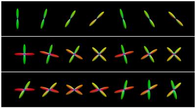
A synthetic dataset consisting of one- and two-directional fiber bundles was generated for quantitative evaluation of the proposed method. The dataset was simulated with $$$b=3000\,\text{s}/\text{mm}^{2}$$$ and 81 non-collinear gradient directions. We generate a set of diffusion signal profiles of fiber bundles oriented according to the Watson probability distribution. Parameter $$$\theta_{\text{T}}$$$ determines the degree of dispersion of the orientations of the fiber bundles. The fiber orientation distribution functions (ODFs) of some diffusion profiles are shown in Fig. 2.

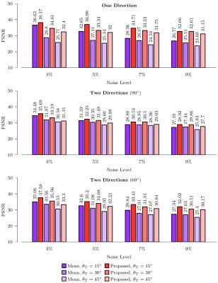
Four levels of Rician noise (3$$$\%$$$, 5$$$\%$$$, 7$$$\%$$$ and 9$$$\%$$$) was added to the dataset. Rician noise was simulated by adding Gaussian noise (i.e. $$$\mathcal{N}(0,v(p/100))$$$) to the complex domain of the signal with noise variance determined by noise-level percentage $$$p$$$ and maximum signal value $$$v$$$ (150 in our case). As shown in Fig. 3, for the various noise levels, our method improves the PSNRs over simple averaging for both cases of one- and two-directional fiber bundles.

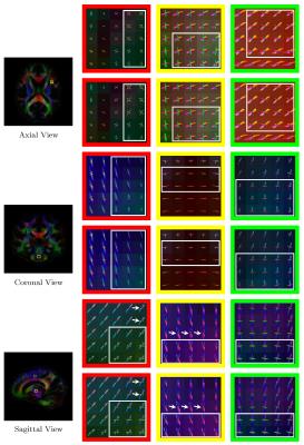
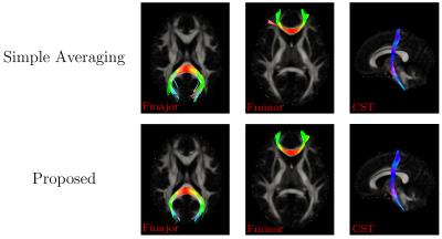
Further evaluation was performed using the diffusion-weighted images of ten subjects from the Human Connectome Project (HCP). Only the $$$b=3\text{,}000\,\text{s}/\text{mm}^2$$$ shell was used in this experiment. Atlas construction was performed after registering the images to a common space with proper signal reorientation⁶. As shown in Fig. 4, our method obtains ODFs that are more consistent with greater directionality. Visible differences as marked using arrows and boxes. Our method gives sharper and longer glyphs, indicating its superiority. Tractography results, shown in Fig. 5, indicate that our proposed method gives cleaner and richer fiber tracts compared with the simple averaging method.

Discussion and Conclusion

Acknowledgements

References

1. Wessel, P. and Smith, W. H., [The Generic Mapping Tools], http://gmt. soest. hawaii. edu (2001).

2. Yap, P.-T., Jiang, X., and Kot, A. C., “Two-dimensional polar harmonic transforms for invariant imagerepresentation,” IEEE Transactions on Pattern Analysis and Machine Intelligence 32, 1259–1270 (2010).

3. Coupé, P., Yger, P., Prima, S., Hellier, P., Kervrann, C., and Barillot, C., “An optimized blockwise nonlocalmeans denoising filter for 3-D magnetic resonance images,” IEEE Transactions on Medical Imaging 27(4),425–441 (2008).

4. Manjón, J. V., Carbonell-Caballero, J., Lull, J. J., García-Martí, G., Martí-Bonmatí, L., and Robles, M.,“MRI denoising using non-local means,” Medical image analysis 12, 514–523 (2008).

5. Comaniciu, D. and Meer, P., “Mean shift: A robust approach toward feature space analysis,” IEEE Trans-actions on Pattern Analysis and Machine Intelligence 24(5), 603–619 (2002).

6. Chen, G. and Zhang, P. and Li, K. and Wee, C. and Wu, Y. and Shen, D. and Yap, P., "Improving Estimation of Fiber Orientations in Diffusion {MRI} Using Inter-Subject Information Sharing," Scientific reports, (2016).