3462
Theory, validation and application of blind source separation to diffusion MRI for tissue characterisation and partial volume correction1Technische Universität München, Munich, Germany, 2GE Global Research Europe, Garching, Germany, 3EMRIC, Cardiff University, Cardiff, United Kingdom, 4CUBRIC, Cardiff University, Cardiff, United Kingdom
Synopsis
Here we present blind source separation (BSS) as a new tool to analyse multi-echo diffusion data. This technique is designed to separate mixed signals and is widely used in audio and image processing. Interestingly, when it is applied to diffusion MRI, we obtain the diffusion signal from each water compartment, what makes BSS optimal for partial volume effects correction. Besides, tissue characteristic parameters are also estimated. Here, we first state the theoretical framework; second, we optimise the acquisition protocol; third, we validate the method with a two compartments phantom; and finally, show an in-vivo application of partial volume correction.
Purpose
The compartmental nature of tissue is generally accepted1,2,3,4,5,6. The diffusion-weighted MRI (dMRI) signal depends on the relaxation times of the compartments (T2i), their diffusivities (Di), volume fractions (fi) and proton density (S0). The simultaneous contribution of these parameters results in a lack of specificity to each independent effect and induces a bias7,8 on the diffusion metrics known as partial volume contamination. Specificity and partial volume correction problems have been addressed independently5,8,9,10,11. Here we present blind source separation (BSS) as a new approach in dMRI that separates mixed signals and yields tissue microstructure parameters, tackling both problems at once.Methods
Theory
This method is based on three assumptions: 1) tissue is made of water compartments with different diffusivities5,9; 2) there is no water exchange2; and 3) each compartment has a different T25,6,9. Hence, we can describe the measured diffusion signal as the weighted sum of the compartmental sources. These weights depend only on the volume fraction (f) and the ratio between the compartmental T2i and the experimental TEj. Therefore, varying TE modifies the weights and the system can be expressed as a BSS problem:
$$\begin{bmatrix}X(TE_1,\Delta,q)\\\vdots\\X(TE_M,\Delta,q)\end{bmatrix}=\begin{bmatrix}f_1e^{\frac{-TE_1}{T2_1}}&\cdots&f_Ne^{\frac{-TE_1}{T2_N}}\\\vdots&\ddots&\vdots\\f_1e^{\frac{-TE_M}{T2_1}}&\cdots&f_Ne^{\frac{-TE_M}{T2_N}}\end{bmatrix}\begin{bmatrix}S_1(\Delta,q)\\\vdots\\S_N(\Delta,q)\end{bmatrix}S_0$$
$$X=AS$$
Where X are the measurements for several TEs, A the mixing matrix, S the compartmental diffusion source, M the number of measurements, and N the number of compartments. Here, among the possible BSS solutions12, and unlike in13, we use a sparsifying transform14 followed by non-negative sparse coding15.
Here we focus on two-compartment environments (N=M=2). Besides, when T2i is larger than the range of TEs (i.e. CSF), the exponential term can be dismissed ($$$e ^{\frac{TE_j}{T2_i}}\approx1$$$) and thus T2i. Alternatively, T2i can be fixed to an expected value if prior knowledge is available (i.e. T2CSF≈2s 6). We study the effect of both approximations on the error of the parameter estimations.
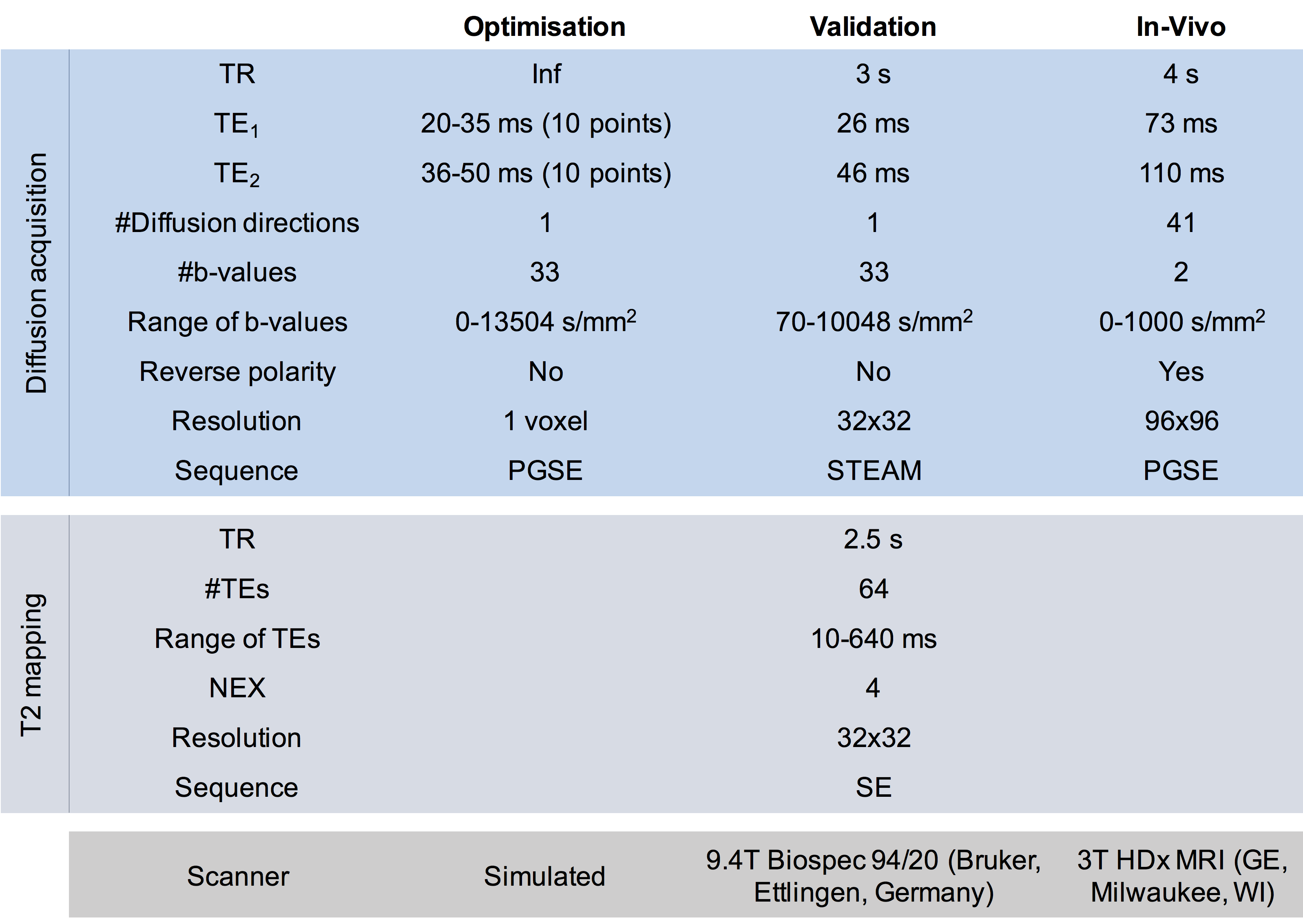
We perform three experiments to: 1) find the range of optimal TEs; 2) validate our method; and 3) show an application. Table.1 contains the experimental details.
Optimisation simulations
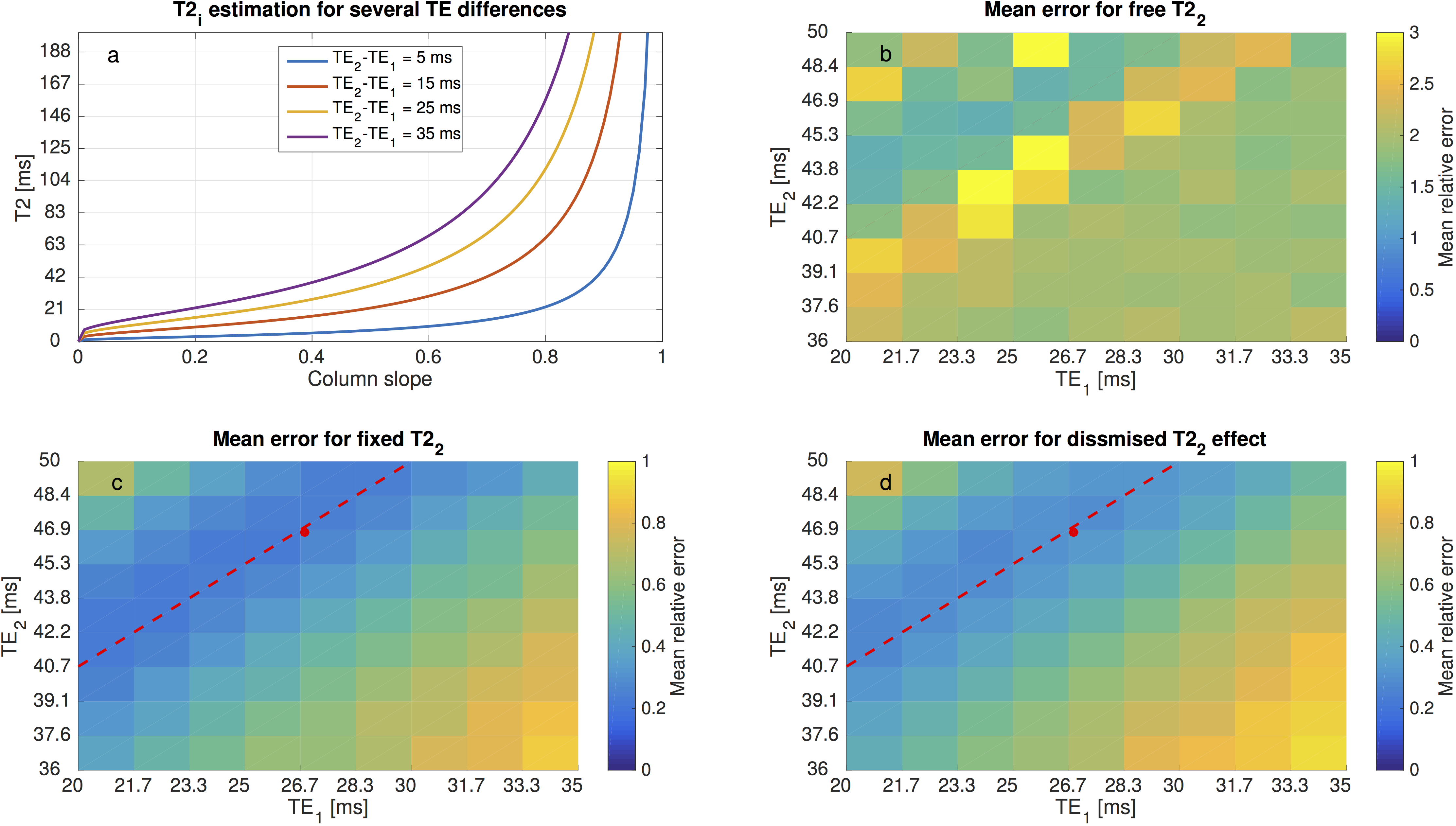
Tissue with two compartments was simulated with known T2s (22 and 597ms) for restricted and free diffusion signals16. We ran a simulation experiment varying TE and f (11 points) to calculate the mean error for all the parameter combinations and find the optimal TE region for free, fixed and dismissed T22.
Phantom validation
For validation, we used a phantom made of yeast and water (1:1) as a two compartments sample17. A multi-echo experiment was acquired and T2s fitted with NNLS18 and EASI-SM19. Besides, BSS was applied on the diffusion dataset fixing T22=0.6s (as estimated by NNLS). Finally, results from the three methods were compared.
In-vivo
A young female volunteer went under a DTI acquisition. CSF signal was extracted from the data using BSS, fixing T22=2s 6. Finally, DTI metrics with and without correction were compared.
Results and discussion
Optimisation simulations
Fig1.a depicts T2 versus the slope of a column of A. As the slope tends towards 1, the estimation falls into an asymptotic region increasing the uncertainty on the T2 estimation. Therefore, fixing its value or dismissing its contribution reduces the mean error of the parameter estimations (Fig.1b-d). Moreover, fixing the T2 value performs slightly better than dismissing its effect (Fig.1c-d).
Phantom validation
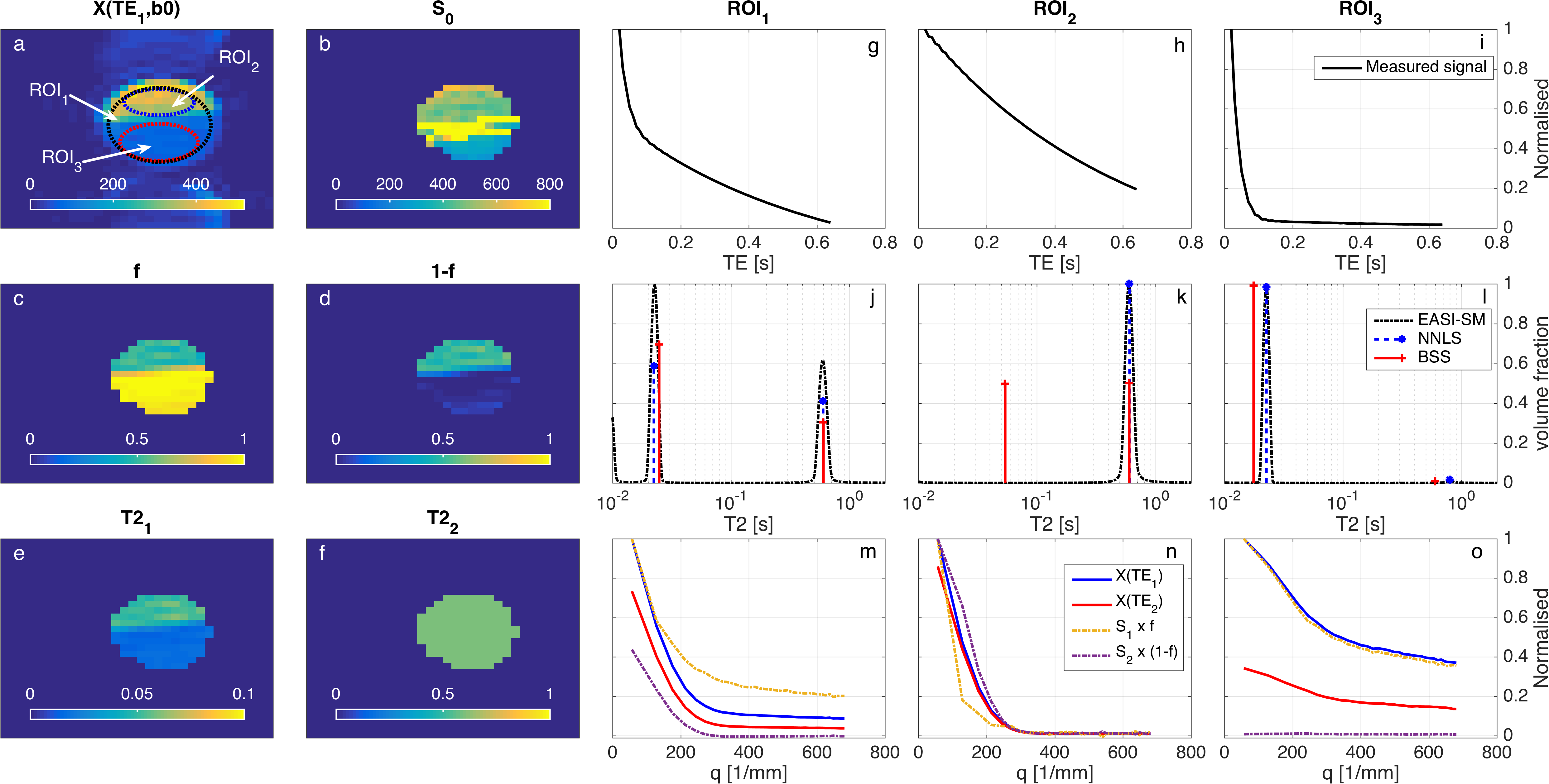
Fig.2g-o compare the results of BSS against NNLS and EASI-SM in a ROI-based analysis. Fig.2j,l show agreement of T21 and f with NNLS and EASI-SM for ROI1 and ROI3. Besides, in Fig.2m, S1 (associated with intra-cellular space) describes a restricted diffusion signal similar as in Fig.2o, and S2 (associated with extra-cellular space) shows a free diffusion behaviour as in Fig.2n. Both findings are in agreement with the simulations and indicate that BSS successfully separates signals from two compartments. Interestingly, BSS disentangles measurements from ROI2 into two similar and equally scaled sources (Fig.2n) indicating that only one source exists. For illustration, Fig.2b-f show that the voxel-based maps generated with BSS are consistent with the ROI based analysis.
In-vivo
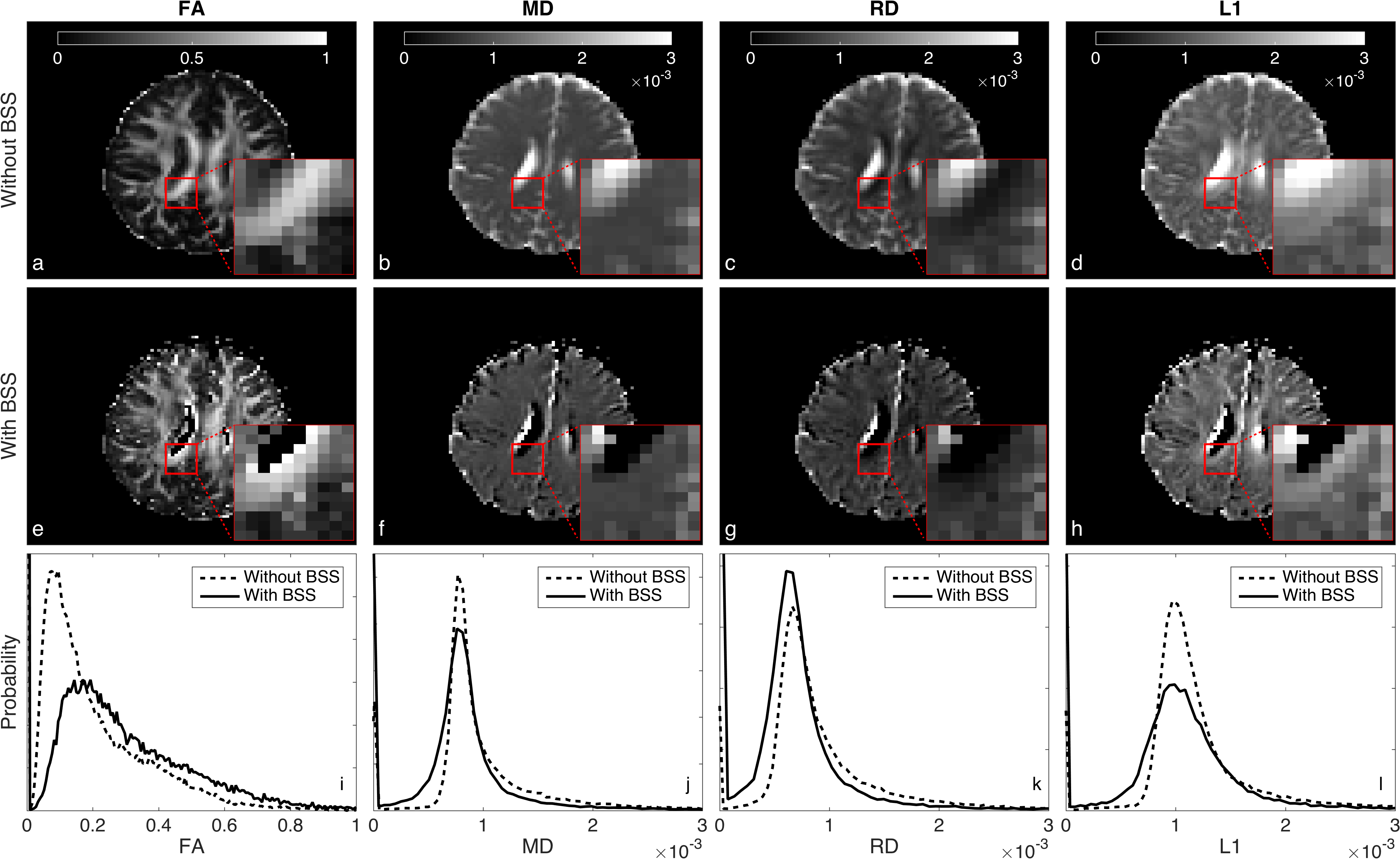
In Fig.3, with BSS, we observe an increase of the fractional anisotropy (FA) (a,e,i) and a reduction of the mean diffusivity (MD) (b,f,j), radial diffusivity (RD) (c,g,k), and tensor’s main eigenvalue (L1) (d,h,l). This is consistent with the elimination of the CSF contribution. Also, we notice that with BSS the ventricles are extracted and white matter structures are better defined, especially the voxels at the border of the ventricles (zoomed area).
Conclussions
Here we show that BSS of diffusion data is a suitable technique to separate compartmental sources. We demonstrate that this method is appropriate for partial volume correction. Besides, tissue volume fraction, relaxation and diffusivity parameters are estimated allowing for simultaneous tissue characterisation.Acknowledgements
With the support of the TUM Institute of Advanced Study, funded by the German Excellence Initiative and the European Commission under Grant Agreement Number 605162.References
1. Stanisz GJ, Szafer A, Wright GA, Henkelman RM. An Analytical Model of Restricted Diffusion in Bovine Optic Nerve. Magn Reson Med. 1997;37:103-111.
2. Assaf Y, Basser P. Composite hindered and restricted model of diffusion (CHARMED) MR imaging of the human brain. Neuroimage. 2005;27:48-58.
3. Zhang H, Schneider T. NODDI: Practical in vivo neurite orientation dispersion and density imaging of the human brain. Neuroimage. 2012;61:1000-1016.
4. Ferizi and others. A ranking of diffusion MRI compartment models with in vivo human brain data. Magn Reson Med. 2014;72(6):1785-1792.
5. Peled S, Cory DG, Raymond SA, Kirschner DA, Jolesz FA. Water diffusion, T(2), and compartmentation in frog sciatic nerve. Magn Reson Med. 1999;42(5):911-918.
6. MacKay and others. Insights into brain microstructure from the T2 distribution. Magn Reson Med. 2006;24(4):515-525.
7. De Santis S, Assaf Y, Jones DK. The influence of T2 relaxation in measuring the restricted volume fraction in diffusion MRI. In: ISMRM. ; 2016.
8. Pasternak O, Sochen N, Gur Y, Intrator N, Assaf Y. Free Water Elimination and Mapping from Diffusion MRI. 2009;730:717-730.
9. Does MD, Gore JC. Compartmental study of diffusion and relaxation measured in vivo in normal and ischemic rat brain and trigeminal nerve. Magn Reson Med. 2000;43(6):837-844.
10. Kim D, Kim JH, Haldar JP. Diffusion-Relaxation Correlation Spectroscopic Imaging (DR-CSI): An Enhanced Approach to Imaging Microstructure. In: Proc. Intl. Soc. Mag. Reson. Med. 24. ; 2016.
11. Benjamini D, Basser PJ. Use of Marginal Distributions Constrained Optimization (MADCO) for Accelerated 2D MRI Relaxometry and Diffusometry. Vol 271.; 2016.
12. Yu X, Hu D, Xu J. Blind Source Separation: Theory and Applications.
13. Molina-Romero M, Gómez PA, Sperl JI, Jones DK, Menzel MI, Menze BH. Tissue microstructure characterisation through relaxometry and diffusion MRI using sparse component analysis. In: Workshop on Breaking the Barriers of Diffusion MRI. ; 2016.
14. Ravishankar S, Bresler Y. l0 Sparsifying Transform Learning With Efficient Optimal Updates and Convergence Guarantees. IEEE Trans Signal Process. 2015;63(9):2389-2404.
15. Hoyer PO. Non-Negative Sparse Coding. IEEE; 2002:557-565. doi:10.1109/NNSP.2002.1030067.
16. Cook PA, Bai Y, Seunarine KK, Hall MG, Parker GJ, Alexander DC. Camino: Open-Source Diffusion-MRI Reconstruction and Processing. In: 14th Scientific Meeting of the International Society for Magnetic Resonance in Medicine. Vol 14. ; 2006:2759.
17. Cory DG, Garroway AN. Measurement of translational displacement probabilities by NMR: An indicator of compartmentation. Magn Reson Med. 1990;14:435-444.
18. Lawson CL, Hanson RJ. Solving Least Squares Problems. Journal of Chemical Information and Modeling. Vol 53:1689-1699; 1974.
19. Zachariah D, Kullberg J, Stoica P, Bj M. A Multicomponent T 2 Relaxometry Algorithm for Myelin Water Imaging of the Brain. Magn Reson Med. 2016;402:390-402.
Figures